Quick Start Guide

Reading time: 10 min

DataGraph is a powerful tool for macOS that lets you create custom graphs using a visual, “no-code” approach. DataGraph uses an object-based process that makes it easy to transfer commands and settings between graphs and files.

To get started, let’s begin with a basic example that will guide you through a 10-step process of creating, formatting, and exporting a single graph.

1. Download and install DataGraph on your Mac.
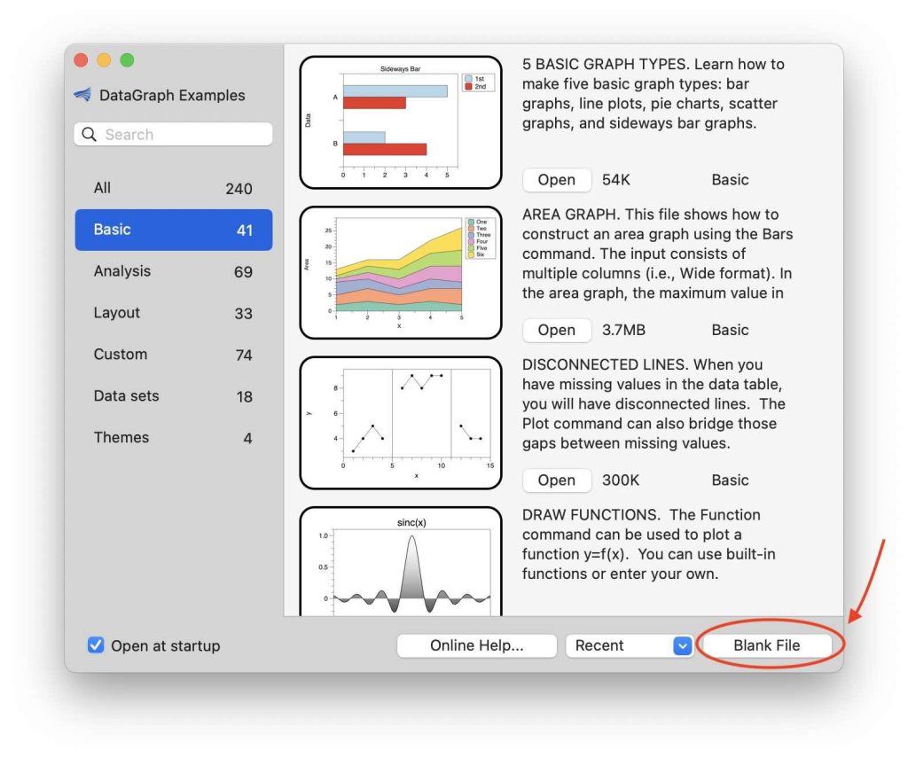
2. Create a new file by selecting “File > New” from the menu bar or clicking “Blank File” on the examples window.
3. Import your data by clicking “Data> Import Data” in the menu bar.
4. Add drawing commands by clicking the “Draw” icon in the toolbar. Find the command you want to use and click “Add.”
5. Specify the input data for each command.
6. Customize each command’s colors, line styles, and more. Expand the command objects for more options.
7. Add commands to annotate your graph by clicking the “Label” icon in the toolbar. Add labels, legends, and more.
8. Customize your graph using the Layout settings to change the size, font, titles, and more.
9. Export your graph by clicking “File > Export Graphic.”
10. Save your Datagraph file by clicking “File > Save” in the toolbar.

Below is a detailed guide for each step and a worked example.

Tip: Exploring the program is a great way to learn how it works. If you make a mistake, use ⌘-Z to undo. DataGraph has unlimited undo from the last time you opened a file. 

1. Install DataGraph

Download and install DataGraph on your Mac. If you do not have a license for DataGraph, you will automatically receive a 7-day trial.

For detailed instructions, see the Installation Guide.

2. Create a New File

Create a new file by selecting “File> New” from the menu bar or by clicking “Blank File” on the examples window (shown below).

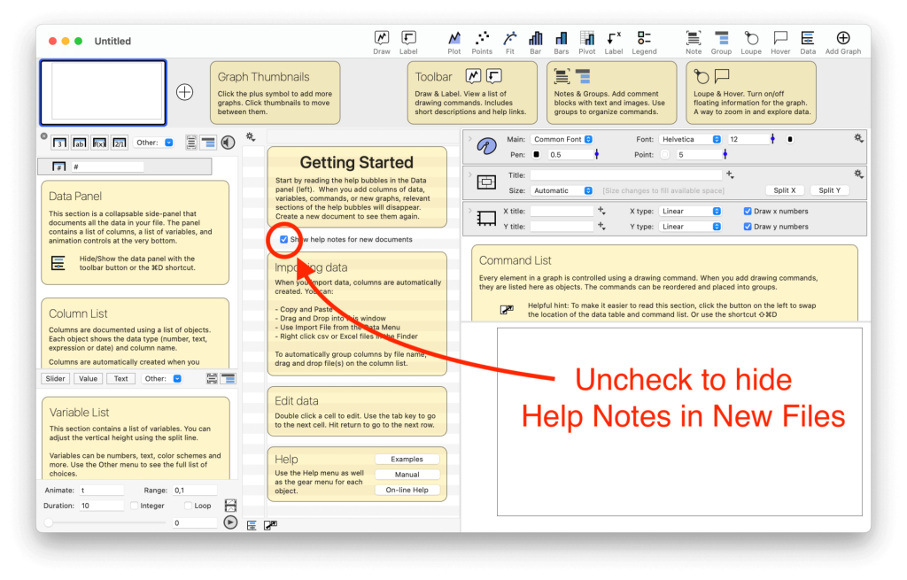
Note: When you create a new DataGraph file for the first time, you will notice a series of help bubbles. As you add elements to the sections, the notes disappear automatically. To stop seeing the help notes, uncheck “Show Help Notes for new documents” as shown below.

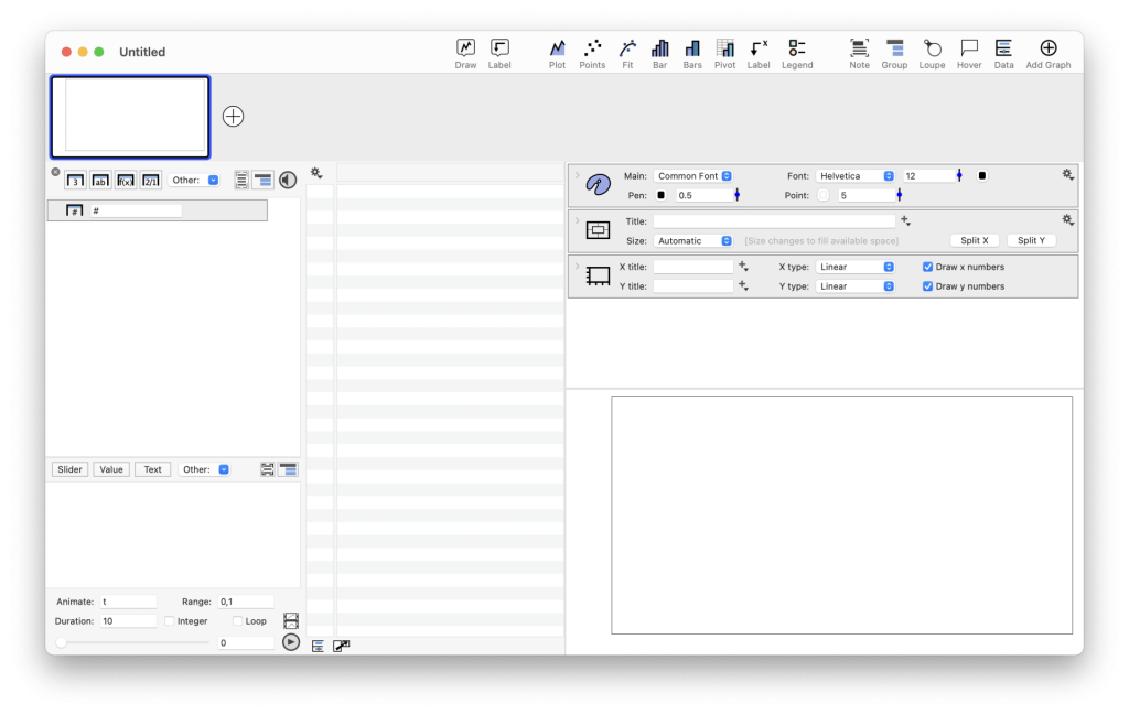
Here is a new blank file.

Learn more about the Examples Files and the structure of the User Interface.

3. Import your data

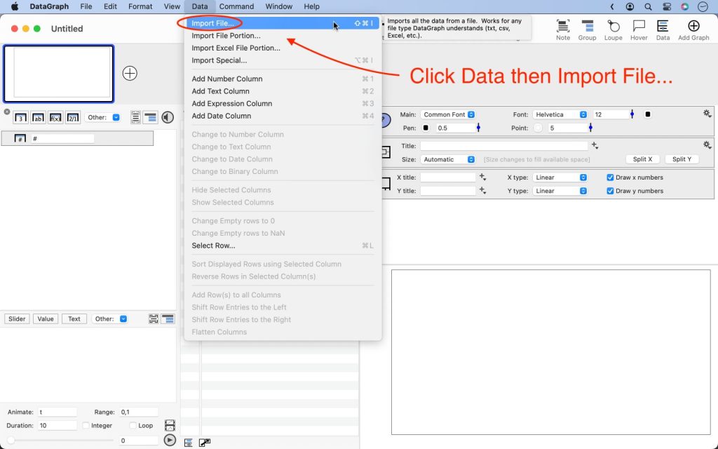
Click “Data > Import File…” from the menu bar (shown below). Use the Finder to select a file.

Example: Download and import: Airmiles.csv. This file contains annual data for passenger miles on commercial US airlines from 1937 to 1960. (Brown, R. G. (1963) Smoothing, Forecasting and Prediction of Discrete Time Series. Prentice-Hall.)

After importing this file, the data table will contain the two imported columns and a built-in row counter. In the data panel, there is an object for each column. The row counter “#” is always at the top.

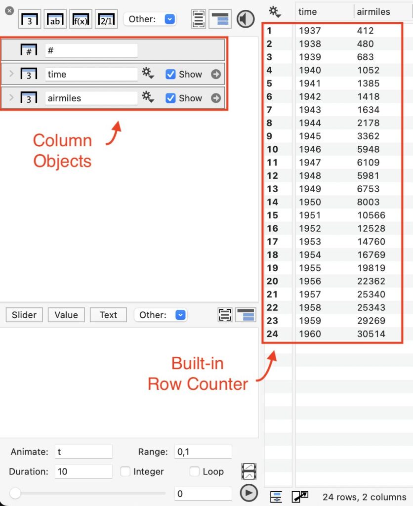
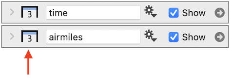
The icon on the left side of the column object indicates the data type. These are both number columns.

Tip: Quickly import CSV/Excel files from the Finder. Control-click the file and choose “Open With > DataGraph”. A new file is created with the data already imported.

**Data Types**: Unlike a spreadsheet, where each cell can be a different data type, in a DataGraph file, the entire column has the same data type. When you import a file, DataGraph assigns each column as Number, Text, or Date.

Number	“3”	Use for arithmetic values to represent a quantity
Text	“ab”	Labels or categorical variables
Date	“2/1”	Dates, time, or time since a given date

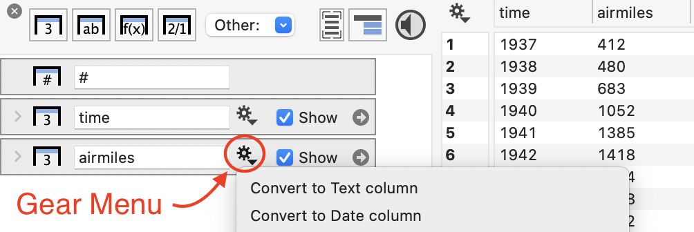
Tip: If the data type is incorrect, click the gear menu on the column object. Select “Convert to …” When you change the data type, you will not change the data, only its interpretation.

Learn more about How to Import Data and the other File Formats you can import.

4. Add Drawing Commands

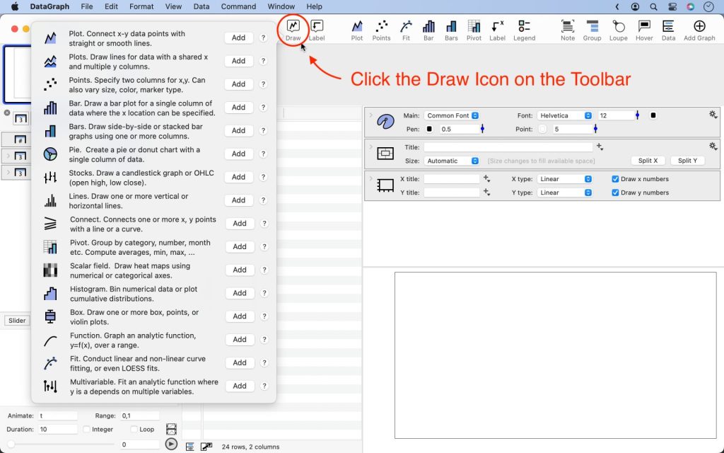
Click the “Draw” icon in the toolbar. Find the command you want to use and click the “Add” button. This adds a command object to the user interface.

Example: Add a Plot command. You will see the Plot command object added to the user interface.

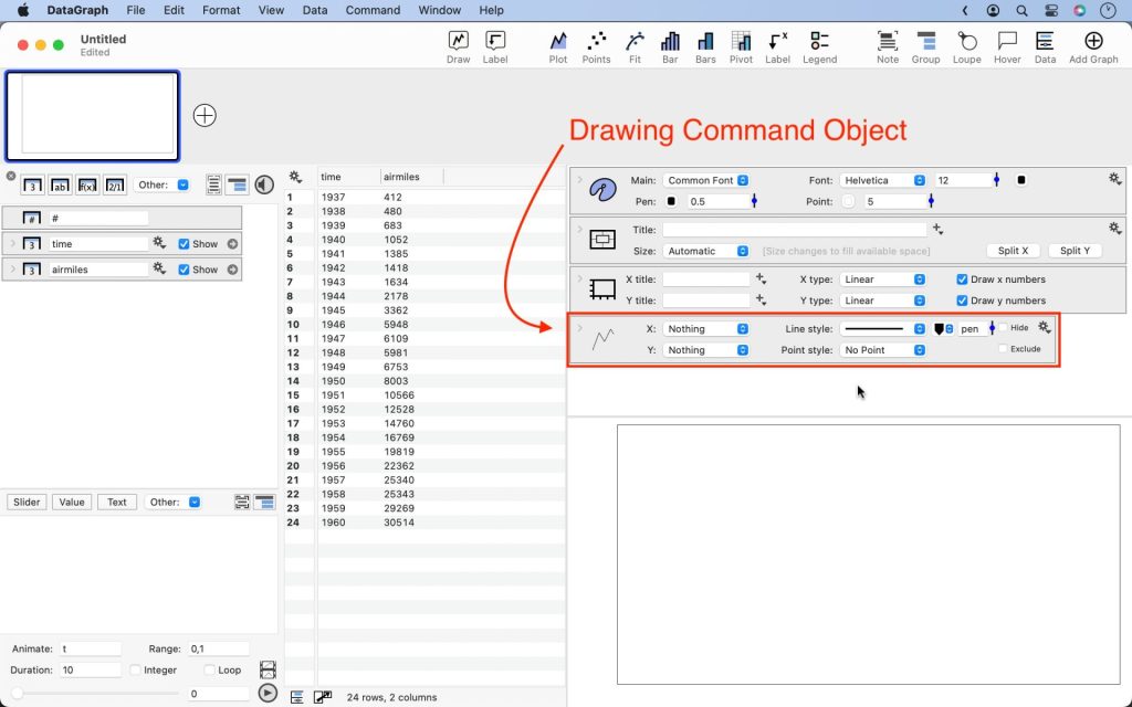
The graph is blank since we have not yet specified the X and Y input data.

Learn more about the commands under the “Draw” toolbar menu.

Plot	Connect x-y data points with straight or smooth lines.
Plots	Draw lines for data with a shared x and multiple y columns.
Points	Draw one point or many. Specify x and y inputs for a scatter graph. Vary size, color, and marker type.
Bar	Draw a bar plot for a single column of data where the x location can be specified.
Bars	Draw side-by-side or stacked bar graphs using one or more columns.
Pie	Create a pie or donut chart with a single column of data.
Stocks	Draw a candlestick graph or OHLC (open high, low close).
Lines	Draw one or more vertical or horizontal lines.
Connect	Connects one or more x, y points with a line or a curve.
Pivot	Group by category, number, month etc. Compute averages, min, max, …
Scalar Field	Draw heat maps using numerical or categorical axes.
Histogram	Bin numerical data or plot cumulative distributions.
Box	Draw one or more box, points, or violin plots.
Function	Graph an analytic function, y=f(x), over a range.
Fit	Conduct linear and non-linear curve fitting, or even LOESS fits.
Multivariable Fit	Fit an analytic function where y is a depends on multiple variables.

5. Specify the Input Data

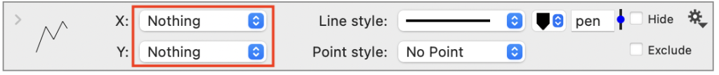
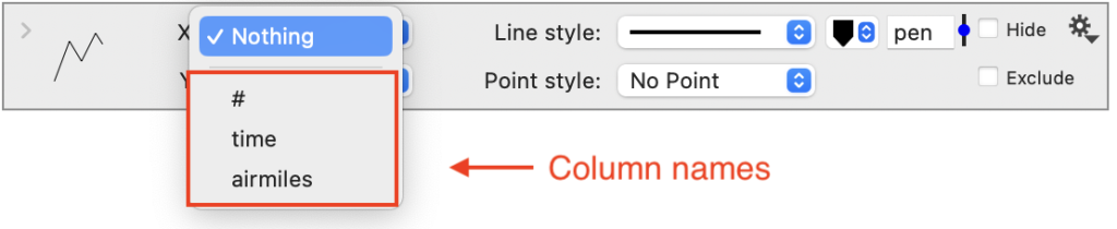
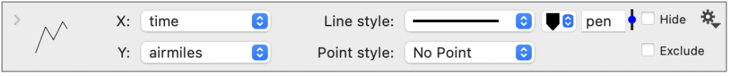
On the command object, click the column selectors to specify the input (e.g., X, Y, Labels, etc.). A scrollable pop-up menu appears, listing the available data columns. Click a column name from this list to select.

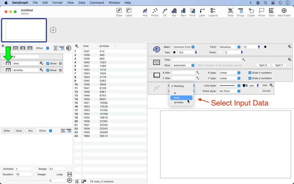
Example: The Plot command needs X and Y inputs. You can select from three columns: “#” (built-in row number), “time”, and “airmiles.”

Set X to “time” and Y to “airmiles.”

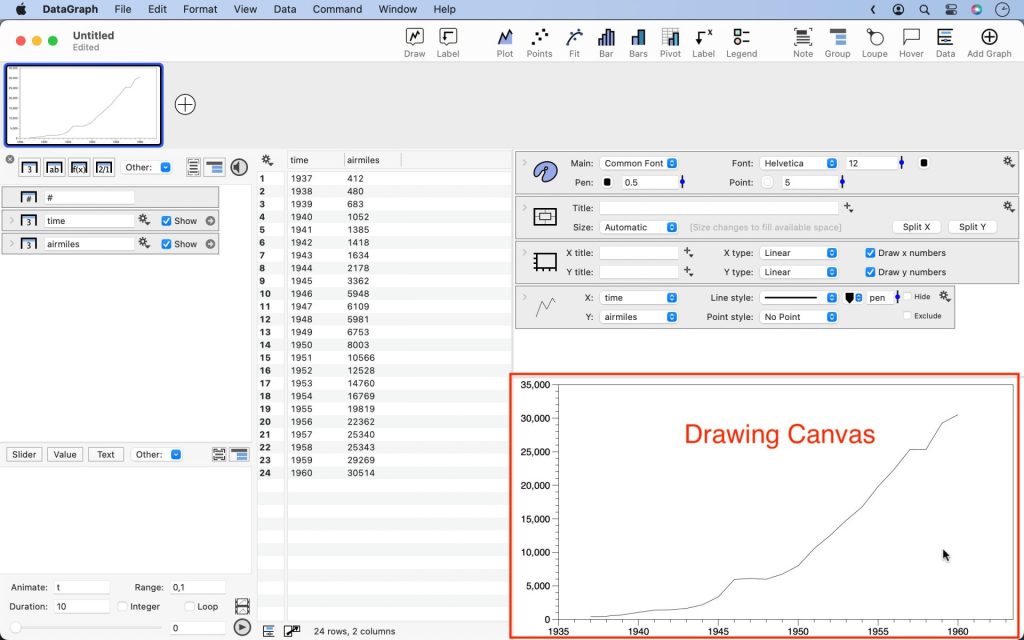
Here is the resulting command and graph.

Tip: If you have the columns selected in the data table and then add the Plot command, the column selectors will be automatically populated. See the video demo in the next section.

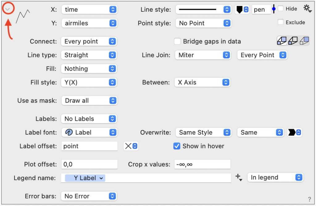
6. Customize Commands

Use the options on the command to change point styles, line styles, colors, and more. Each command will have different options, but many of them share common features.

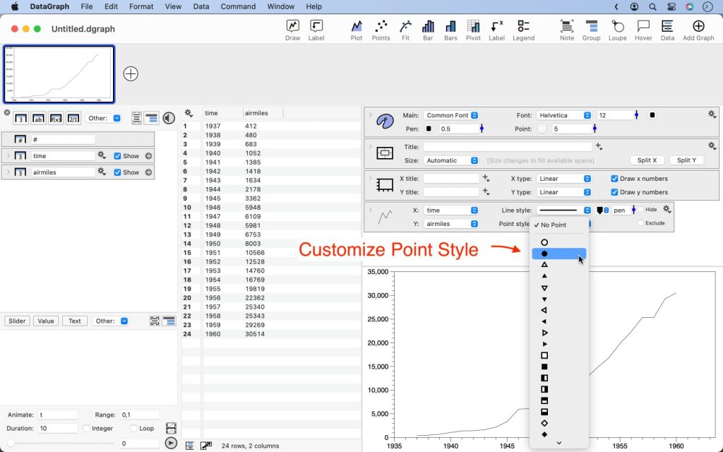
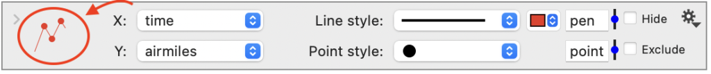
Example: Add points and change the color to red.

1. Click the Point style menu and change from “No Point” to a solid marker.
2. Click the color tile to the right of the Line style to select a new color.

Notice how the graph and the command icon update as you make these changes.

Video Demo: In this demo, the data columns are selected before adding the Plot command from the toolbar. This automatically populates the menu selectors when the command is added. Many commands have similar shortcuts to simplify the graphing process.

Note: Each command shows several key options in the main view but many more options in the expanded view. Click the top left corner to expand a command and see all available options. 

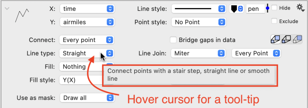
Tip: Hover your cursor over an option or setting. After a moment, tooltips will appear, as shown below for Line type.

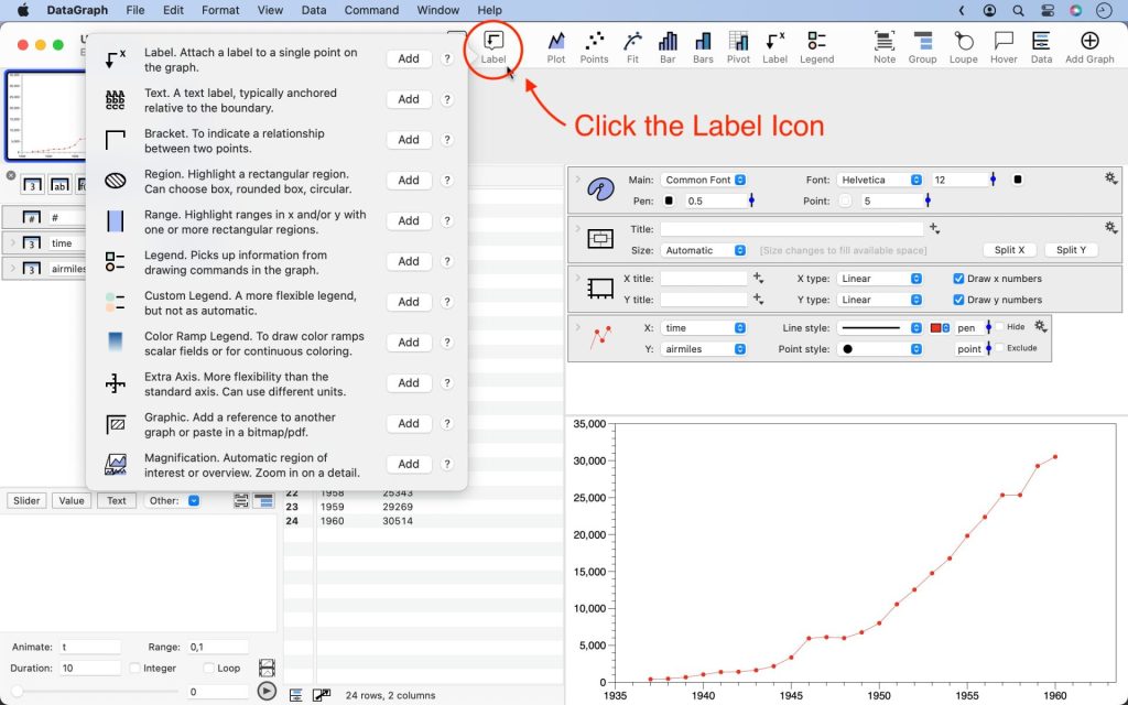
7. Annotate your graph

Click the “Label” toolbar icon for a list of commands to annotate your graph. You can add legends, labels, highlighted regions, and more here.

Example: Add a Label command. The Label command object is added below the Plot command.

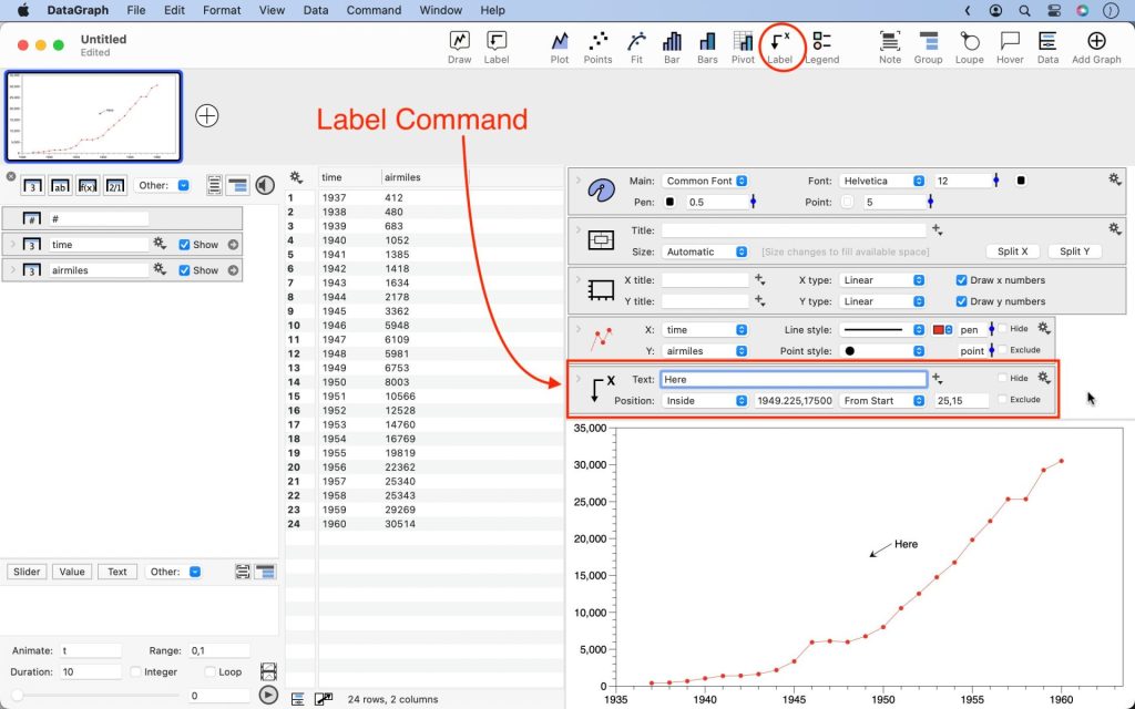
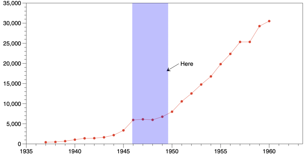
On the graph, an arrow with a text label is added at the center of the graph.

Edit the Label command settings to point at x = 1946. There are three entry boxes to edit. Here is description of each.

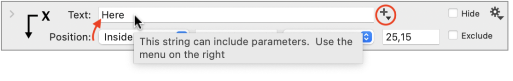
1. Enter text or add parameters as tokens. For this example, we will use the tokens. Click the “+” symbol on the right for a list of available parameters. Select the “X Value.”

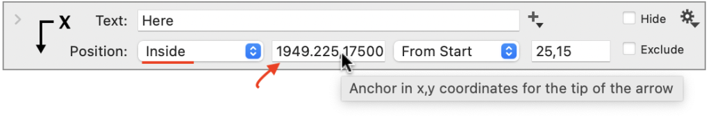
2. Edit the anchor point, the “x,y” location where the arrow is pointing. Set to “1946,5948”.

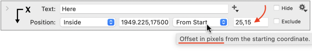
3. Set the label offset, the distance from the anchor to the text. Here, the units are pixels. Set to “0,40”.

Demo: See how to edit the text, move the arrow, and adjust the offset directly on the graph. The corresponding command settings update automatically.

Tip: Avoid zooming accidentally by not dragging too far from the label. If you see a purple region, you’re zooming. Move the mouse back to start to avoid zooming. Use ⌘-Z to undo zooming.

Note: Similar to the label, most commands for annotating your graph add elements that can be positioned interactively by dragging on the graph.

Learn more about the commands under the “Label” toolbar menu.

Label	Attach a label to a single point on the graph.
Text	A text label, typically anchored relative to the boundary.
Bracket	To indicate a relationship between two points. Draw straight or curly braces.
Region	Highlight a rectangular region. Can choose box, rounded box, circular.
Range	Highlight ranges in x and/or y with one or more rectangular regions.
Legend	Picks up information from drawing commands in the graph.
Custom Legend	A more flexible legend, but not as automatic.
Color Ramp Legend	To draw color ramps scalar fields or for continuous coloring.
Extra Axis	More flexibility than the standard axis. Can use different units.
Graphic	Add a reference to another graph or paste in an image file (e.g., bitmap or pdf).
Magnification	Automatic region of interest or overview. Zoom in on a detail. Create an inset.

8. Format the Graph Layout

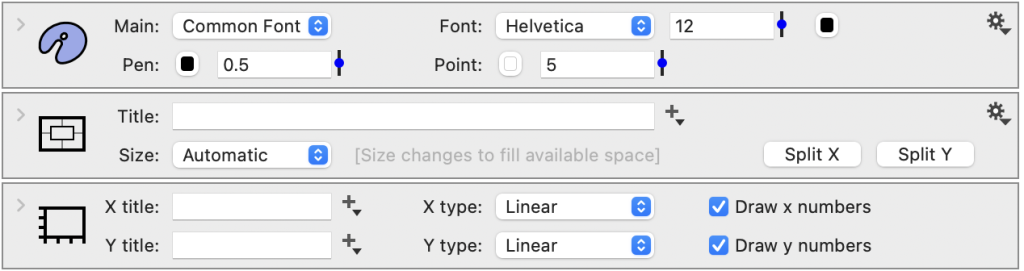
The settings to format your graph are called the “Layout Settings.” They are organized into three objects: Style, Canvas, and Axis settings.

The Layout settings are the control center for your graph. It’s worth spending some time to learn more about the Layout Settings and Split-Axis functionality.

Style settings	Control font, color pallets, gridlines.
Canvas settings	Control size, background colors, margins.
Axis settings	Control tick mark locations, and axis labels.
Split X-Axis	Create graphs with a shared X axis.
Split Y-Axis	Create graphs with a shared Y axis.

Where to start? We recommend setting the graph size first. Other key settings are the font size, adding a title, and axis labels. The number of tick marks and gridlines will adjust automatically based on these settings.

Example: Follow along to change the size, font, box style and more.

1. Graph Size: Click the “Size” menu on the Canvas settings and change to “Specified.” An entry box appears to the right. The default value is “5in,3in”.

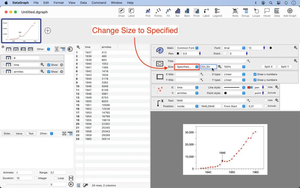
Tip: The graph size is now fixed and will not fill the area within the sliding bars, but you can change the zoom. Learn more about How to set the Graph Size.

Note: Sizing and distances that look proper in the screen resolution may look large when the image is sized correctly. For example, once the size is set, the label looks too far from the data.

To improve the appearance, change the y offset on the Label command from “0,40” to “0,20”.

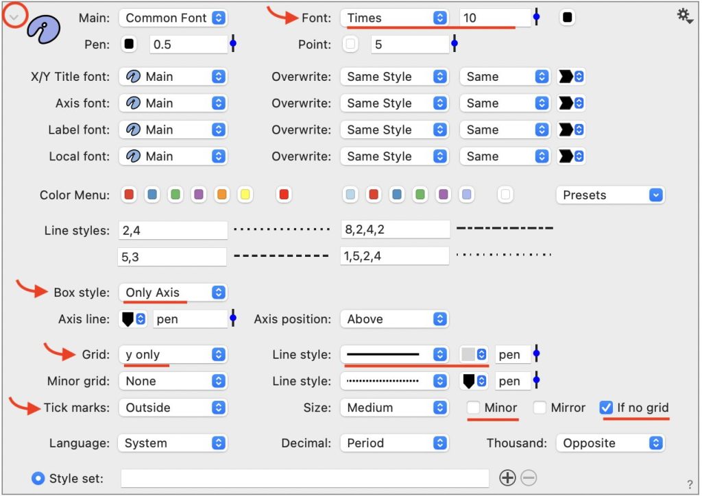
2. Font Size: Change the main Font on the Style settings. Change Font to “Times” and the Font size to “10”.

When the font is smaller, the margins decrease slightly, and the automatic formatting allows for more tick marks.

3. Box style, Grid, and Tick marks: Click the top left corner to expand the Style settings and see all available options. Try them out!

Here we changed the following settings:

• Set Box style to “Only Axis”.
• Set Grid to “y only” .
• Set the Line Style for the grid to a solid, grey line.
• Uncheck “Minor” to remove minor tick marks.
• Check “If no grid” to show tick marks, only when there are no gridlines.

Here is the graph now.

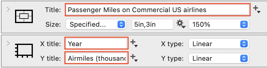
4. Add Titles: Use the text boxes on the Canvas and Axis settings to enter a graph title and axis titles.

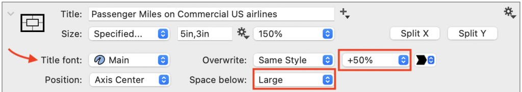
• Set the Title to “Passenger Miles on Commercial US airlines”
• Set the X title to “Year”
• Set the Y title to “Airmiles (thousands)”

The graph has titles now, but with the font the same size, the title looks small relative to the numerical axis labels.

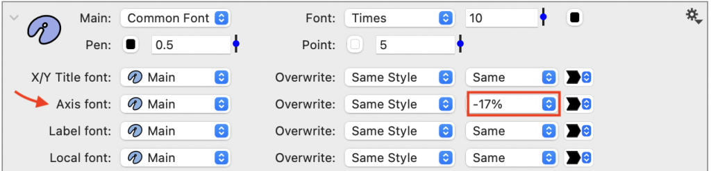
5. Adjust the Relative Font size. DataGraph has a convenient feature that lets you adjust the font up or down relative to the main font size.

Adjust the Axis font down in the Style settings. Notice the other font groups that can be formatted here.

Adjust the Title font up in the Canvas settings. You can also add space below the title.

We are done! The graph looks more balanced and complete after adjusting the font sizes.

9. Export your Graph

Click “File” in the menu bar and select “Export Graphic.”

Example: You don’t need to export a separate graphic file but can copy and paste the image directly into a document or presentation.

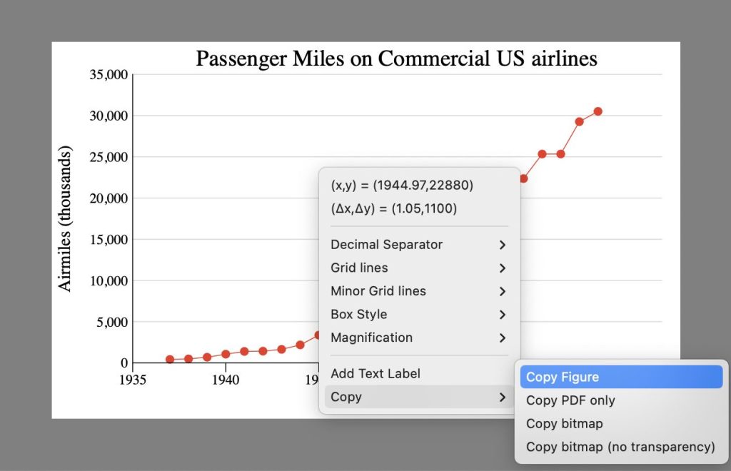
To quickly move a graphic to another program, control-click on the graph and select “Copy > Copy Figure” (shown below). Next, paste the image directly into its destination.

**Important**: If you resize your graph in another program, you will change the font size. Thus, the font size you selected in DataGraph will not be maintained. For the best quality and consistency, update the size in DataGraph and then reimport the image.

Learn more about How to Export An Image.

10. Save your File

Click “File” in the menu bar and select “Save.” This will allow you to come back and edit your graph later if needed.

Learn more about Saving Files.

Summary

You have learned the basic process of creating a graph in DataGraph from this webpage. In the beginning, we mentioned that DataGraph makes transferring commands and settings between graphs and files easy.

Here is a final demonstration. See how to transfer commands/settings from one graph to another:

Why does this work? When you transfer commands from one file to another, the commands will search for columns with identical names to use as input. The columns don’t need to be in the same order but must have the same name. If the names differ, you must manually select the input data.

Try it yourself!

1. Make a new DataGraph file.
2. Import Airmiles.csv.
3. Go to the DataGraph file where you already created a graph.
4. Click and drag to the side of the commands/settings to select them all.
5. Select Edit > Copy. This copies the commands/settings to the clipboard.
6. Go back to the new DataGraph file.
7. Select Edit > Paste to copy the commands/settings to the clipboard.

You created a new graph with all the same settings using a simple copy & paste! You can highlight any combination of settings and commands to move them between graphs and files. 

Questions, Comments, or Feedback?: Click “Help” in the menu bar. From here, you can email us directly or set up an account for the Forum.