Plot

The Plot command is used to drawn lines between x and y corrdinate locations.

Input

The Plot command requires two columns, X and Y.

These can be number columns, date columns, or text columns.

NEW: In DataGraph 5.2, you can use text columns as input. The text labels the axis in categories, and the underlying numerical location is the row number.

Options

The command includes options for how the connection between the points is represented, adding fill styles, labels and more.

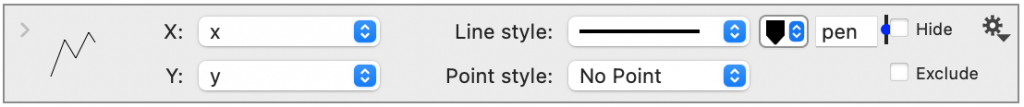
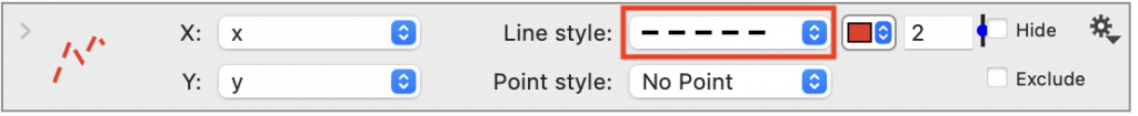
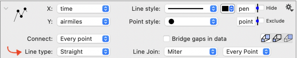
Line Style

By default, the command draws a solid line, that has the same color and width as the pen in the Style settings. You can modify the line style, color, and width. Choose from the nine built-in line styles.

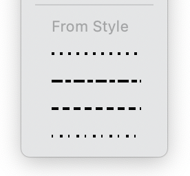
At the bottom of the Line style menu, there is a section labeled ‘From Style’. These are styles that you can customize in the Style settings.

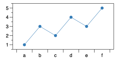
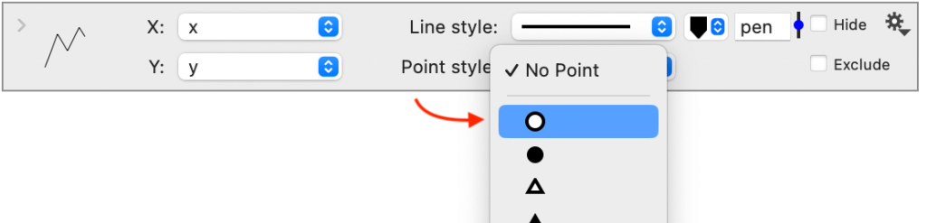
Point Style

You can add points at the x-y coordinates. There are over 20 different points styles to choose from. The makers alternate between symbols with an open fill and a solid fill.

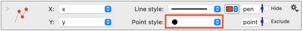
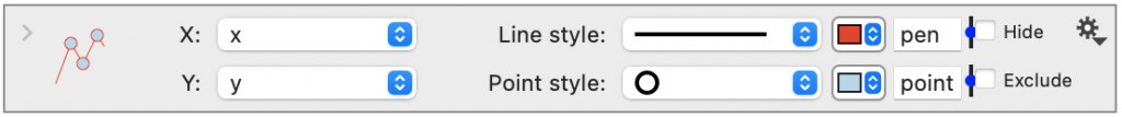
Solid Marker

For solid points, the point and line color are the same.

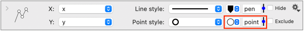
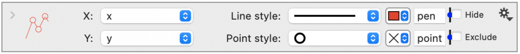
Open Marker

If you select any symbols with an open marker, a color menu and an entry box appear to the right. The color menu controls the fill color, and the entry box controls the marker size.

The fill color is initially set to the predefined point color in the Style settings, but you can change it to any of the colors in the menu or use the color picker.

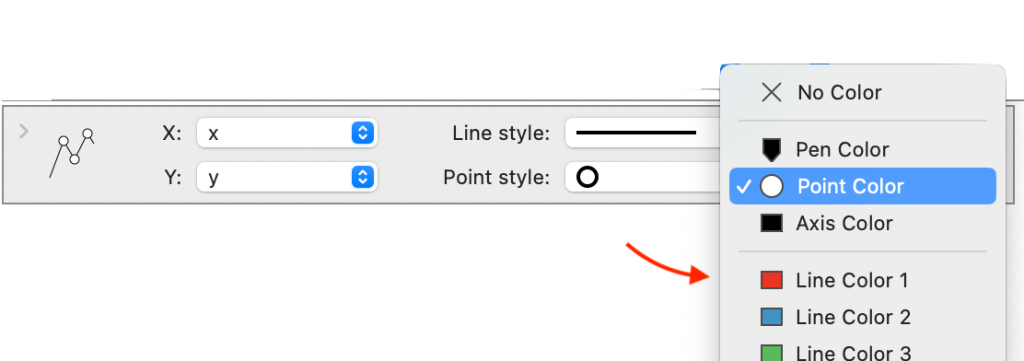
You can change the fill and line color independently, but the marker’s outline will always match the color of the line.

You can also select ‘No Color’ from the color menu. This means the fill is transparent such that overlapping points, other graph elements, or background colors set in the Canvas settings can show through.

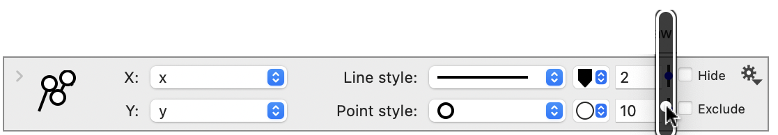
Marker Size

The entry box is set to the variable “point” by default. You can change the value of “point” in the Style settings to change it everywhere the variable is used or change the value on the command itself.

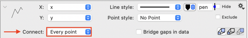
Connect

The connect setting allows you to draw multiple disconnected lines, even when your data points are the same columns. For example, here are two columns of data, where the x values are repeated.

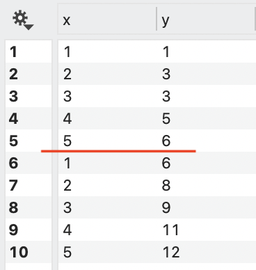
With the default settings, the lines would connect every point.

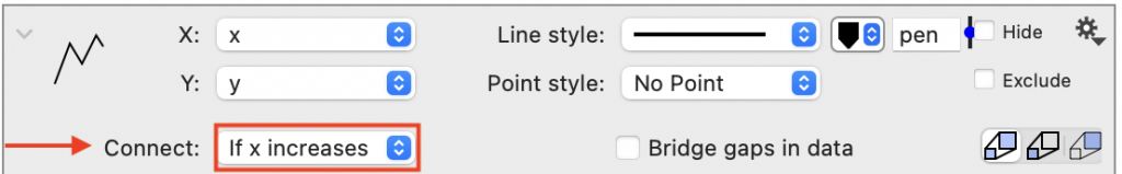
By changing Connect to ‘If x increases’, these are drawn as two lines.

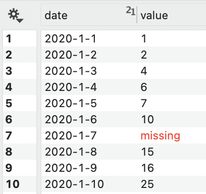
Bridge Gaps

When data is blank or missing from a row, this results in a break in the connection.

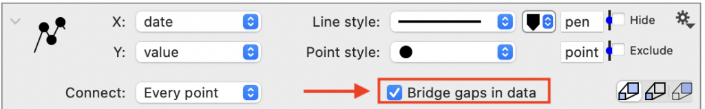
Check Bridge gaps in data to draw the line between the break.

Line Type

The Line type can be Straight, Smooth, or Steps.

If you chose Steps, you can also vary the orientation of the step, relative to the point.

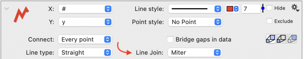
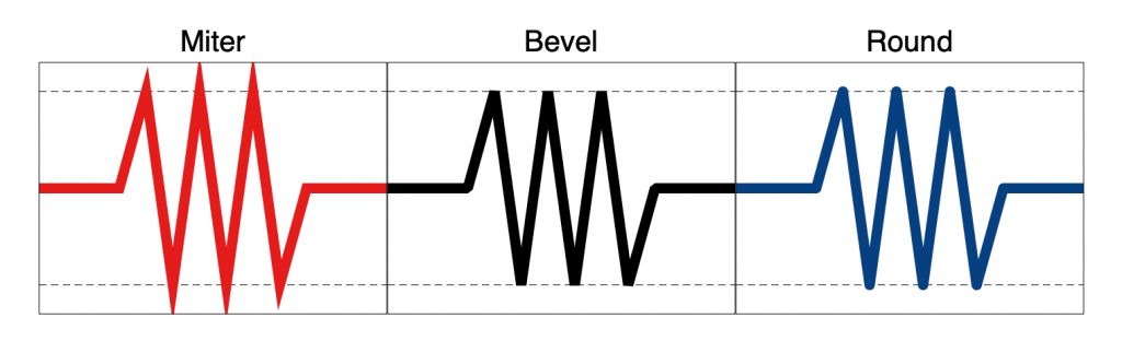
Line Join

The Line Join option controls how line segments are connected. This option is useful when plotting noisy data along with a thick line width. In that case, the connections between the line segments may have spikes with the default setting of ‘Miter’. Change to a ‘Bevel’ or ‘Round’ option to avoid the line connections going beyond the data values.

Fill

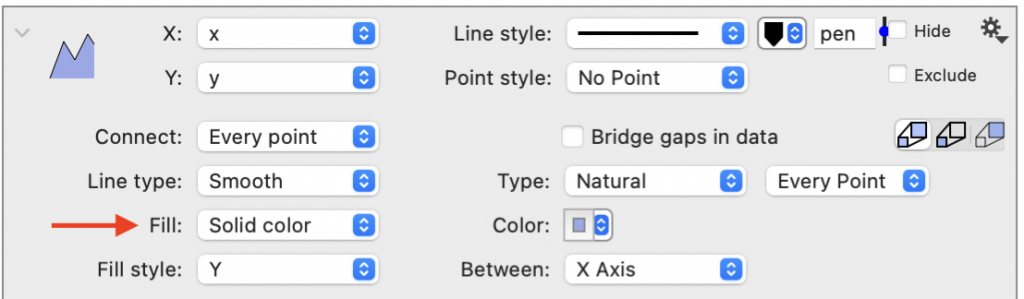
The Fill menu is set to ‘Nothing’ by default. It can be changed to’ Solid, Pattern, Gradient, or Noise’.

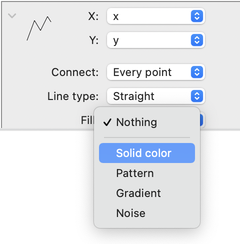
For example, here, the fill is a solid color and fills the area below the line to the X-axis. Options for customizing the fill are displayed to the right of the fill menu and can be changed depending on the selection.

Fill Style

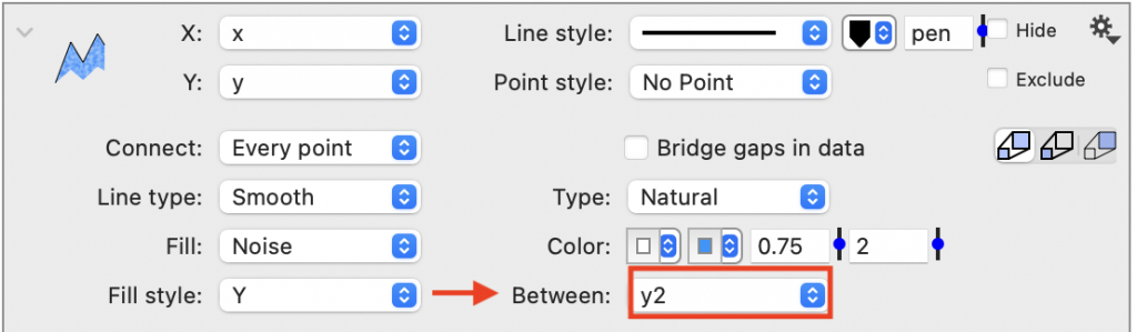
The Fill style can be used to change the direction of the Fill or you can select a column of data. For example, here is data for x and y, along with another y2 column.

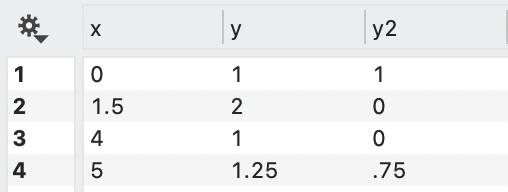
The Fill style is modified so the fill goes between the lines for y and y2. Here the Fill type is ‘Noise’.

Mask

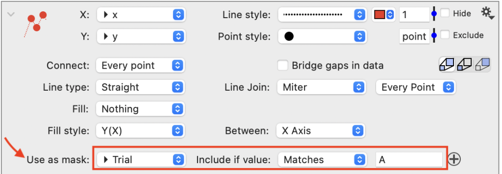
Below the Fill is the Mask option which allows you to filter your data.

Example 1

Here you have a set of data where ‘Trial’ can be ‘A’ or ‘B’.

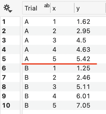
To plot only the ‘A’ set of data, set Use as mask to ‘Trial’ and If value to ‘Matches’. The type ‘A’ as the criteria.

Here is the resulting graph.

To Plot both A and B in the same graph, use a separate command for each.

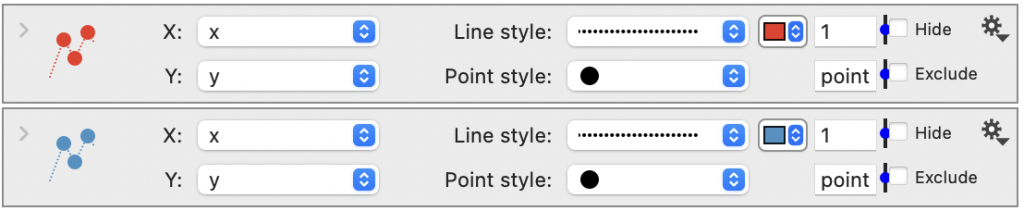
Note: In the above graphs, the Legend name is also set to ‘A’ or ‘B’ and a Legend command has been added.

Example 2

In Example 1, the data was sorted in the same column we used as the mask. If your data is not sorted according to the column you are filtering on, you may have gaps in your line, or no line at all.

The solution could be to sort your data, but often it is good practice not to modify your original data set, and instead you can use the Bridge gaps check box disscussed above.

For example, here you have data that alternates between ‘A’ and ‘B’.

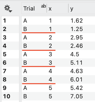
Plotting all the data will result in both A and B being shown.

As in Example 1, we can add a Mask to show the points only when the column ‘Trial’ matches ‘A’; however, the masked rows (i.e., in this case, where Trial matches ‘B’) are treated as blank, resulting in gaps in the connected line.

If you check Bridge gaps in data (See section above), the points will be connected.

Thus, you are able to get a single line from the masked data, without having to do any manipulation of the original data set.

Labels

Below the mask is the label option. This allows you to label each point on the graph.  

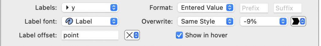
The default Label offset is ‘point,’ a variable defined in the style settings. The Label offset can either be a single value or a coordinate (x,y). If the offset is a single value, DataGraph tries to figure out how to offset the number so it won’t overlap the line. If you specify two values, this offset is used at each point in the x and y direction.

Plot Offset

Shift the (x,y) coordinates. Set to (0,0) by default.

Crop x values

Crop the data without affecting the axis range. Set to -∞,∞ by default.

Legend name

Add a Legend command to show the plot as a legend entry. The default legend name is set to the name of the y column using a token.

You can overwrite the legend name with text or a different token. You can also change the legend location from ‘In legend’ to ‘At the end’.

NOTE: When the legend location is ‘At the end,’ the Label offset is used to set the exact location. Thus, modify the label offset to adjust the location.

Error bars

At the bottom is the error bar selector. By default, it is set to ‘No Error,’ but several entries are in that menu.

For a detailed description, see: How to add Error Bars.

Output

The Plot command does not compute any values for output, but you can use the gear menu in the top right corner to output a column of 1 or 0 to indicate rows included or excluded from a mask.

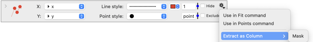
If no mask is applied, you will not see this option.