Fit

The Fit command allows you to fit x-y data with a function and includes linear and non-linear regression (i.e., curve fitting).

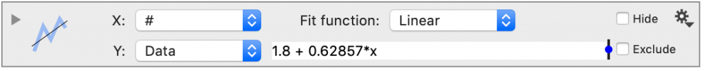
Select the fit function, get the expression, and see the result on the screen. Opening the drawing command reveals a number of options and settings. Some of them are for customizing the visual display of the fit, but many are intended to help you understand the quality of the fit.

Background

The fit works by minimizing a term of the form

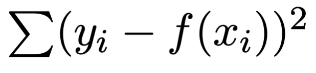
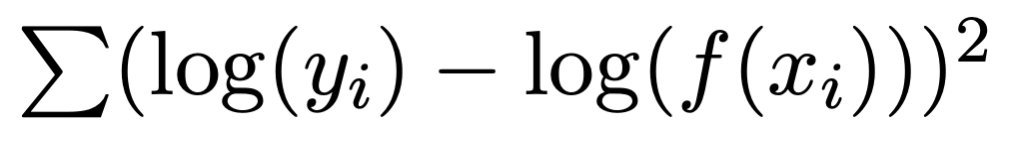
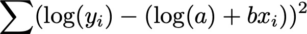
where the function, f, depends on the parameters that you want to optimize. The exception is the exponential and logarithmic fit, where the routine minimizes:

You can specify a weight column, such that each term is weighted by the corresponding row in the weight column. In this case, the term that is minimized is:

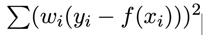
Thus, where the weight is larger, relative to other points, the error is smaller.

Types of Errors

The question may arise why you sometimes minimize the difference of values and sometimes the difference of the log of the values. For the exponential and power fit, taking the logarithm converts a non-linear problem into a linear problem which is much easier to solve mathematically, and was a significant benefit when computers were not as powerful as today.

However, there is another fundamental difference. When you are subtracting the values, you are minimizing the absolute error. While subtracting the log of the values, means you are minimizing the relative error for the fit.

To explain why that is the case, let’s define some notation to make this easier to explain. Call the data values y, the fit result f, and the error e. They are related to the equation

This means that for the standard fit, you are minimizing

If you take the log of the y values you are minimizing

We can manipulate the term inside the square to get

The ratio e/f is the relative error while e is the absolute error. In general for log(1+x), if x is small, log(1+x) is approximately x. Thus, we can show that minimizing the log of the y values is minimizing the relative error.

In practice, minimizing the relative error is useful when the y values span several orders of magnitude, helping to ensure that the residuals for small values have a small relative error. This is helpful for exponential growth and decay, which often spans many orders of magnitude. For the Arbitrary fit option, you have the choice of minimizing y on a linear or logarithmic scale.

Input

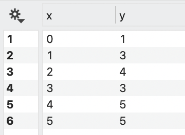
The Fit command requires two numeric columns of data as input, one for the X and one for the Y.

A shortcut is to first create a Points command using the data you want to fit. Next, click the Fit command. The X and Y columns will automatically be populated and the equation for the linear fit is shown in the Fit command.

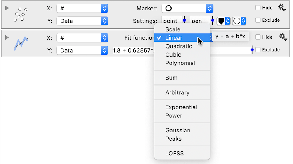
Fit function

Select the form of the equation for conducting the fit. Hover your cursor over the first five options to see the general form of the equation.

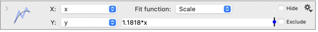
Scale

Chose Scale for a linear fit that goes through the origin (0,0).

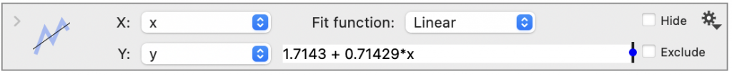
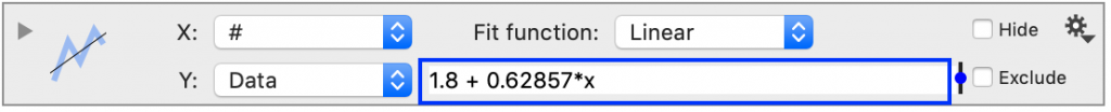
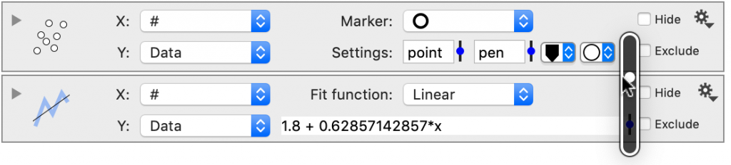
Linear

The Linear fit is a standard linear regression, fitting the slope and the intercept.

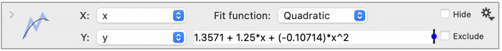
Quadratic

Quadratic results in a second-order polynomial.

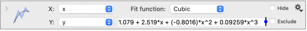
Cubic

The Cubic is the third-order polynomial.

Polynomial

The Polynomial option allows you to fit higher-order polynomials. To the right of the menu, you can specify the order and a slider where you can dynamically change the order.

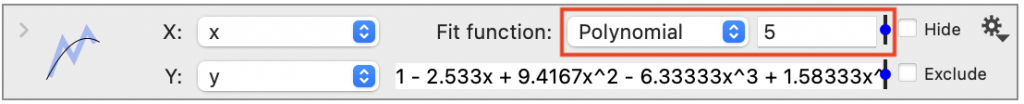
NOTE: For high-order polynomials, the coefficients themselves don’t generally have a lot of meaning or predictive capability, but the approach can be useful for showing trends. To most accurately evaluate a high-order polynomial, use the Plot action column ‘Evaluate’ option.

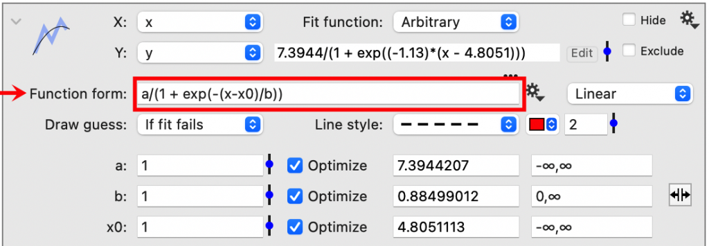
Arbitrary Fit

The Arbitrary Fit allows you to specify a function with unknown parameters. DataGraph computes the parameters to minimize the difference between the function and the data.

Mathematically, the arbitrary fit is referred to as generalized least squares, or non-linear least squares, and allows you to specify a non-linear function. Unlike a linear function where there is a unique solution, non-linear functions may have multiple solutions. An iterative process is used to find the fit and might find one of the solutions, or not converge at all (See Levenberg–Marquardt algorithm on Wikipedia for more details).

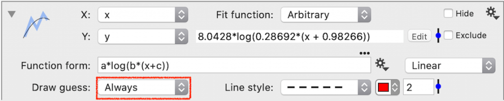
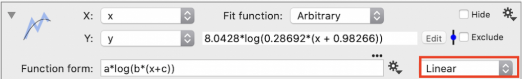
Function form

You can include global variables and use any of the built-in functions (See the Function Reference). Enter the function in the Function form entry box, and the unknown coefficients will be listed below. In this example, the unknown coefficients are a, b, and x0.

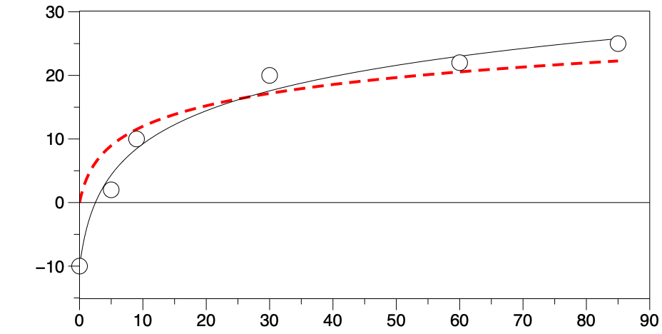
Draw Guess

DataGraph allows you to specify an initial guess for each parameter. The default guess is the number ‘one’, but you can vary this guess by typing in a new value or by using the pop-up slider.

Typically, better fits are obtained when the initial guess is close to the function. A quick way to assess the values of the initial guess is to set Draw Guess equal to ‘Always’.

Linear vs. Logarithmic

To the right of the Function form, there is a menu to choose ‘Linear’ or ‘Logarithmic’.

Linear is the default approach that minimizes (data – y) or absolute error. Logarithmic changes the fit to minimize log(data) or relative error. See the section on Errors for more information. For data spanning several orders of magnitude, the fit may have difficulty converging using the Linear option. In this case, try the Logarithmic setting.

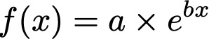
Exponential

The Exponential option fits data to an exponential function, without you having to log transform the input data to use a linear fit option.

The Exponential option fits the equation,

DataGraph fits the linearized form of the equation, using the natural log, such that

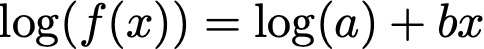
The coefficients are determined by minimizing the equation

Using this approach minimizes the relative error as discussed above.

Two coefficients are provided in the fit output where a is the scale and b is the power. The default legend shows the equation and coefficients.

On the Axis settings, change the Y type to ‘Logarithmic’ to view the fitted curve as a straight line.

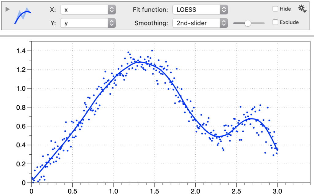
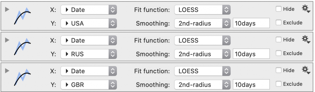
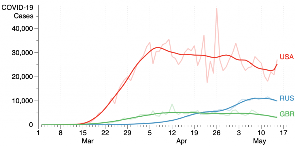
LOESS

Use the LOESS option to smooth data that does not fit an analytic function.

LOESS uses a weighted least squares fit in a specified window. Using the Smoothing menu, chose either 1st or 2nd-degree polynomials. The window can be explored using a slider or specified with an expression.

You can adjust the size of the window through a slider. The slider goes through a predefined range of values and is in terms of the width of the range of x values.

Change the smoothing to use the radius and you can set the range with an expression.

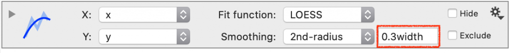
In this field, the “width” value is defined to be the width of the interval, the same as the slider uses. You can get the same effect as the slider by specifying this to be “c*width”, and defining “c” as a variable using a slider. This would allow you to use the same width for several fits, or to animate the fit in time (and save it into a movie).

For the expression, you can specify radius in terms of “minute”, “hour”, “day”, “week”, “month” (singular and plural), so the number “3weeks” is understood as 3 weeks, where weeks is 724*3600 (seconds). This is intended for making it easy to apply a smooth fit for data that is given in terms of dates. It is also possible to define your own constant as a variable.

Fit Results

The Fit results are shown in a window on the main view of the command.

The resulting window can be highlighted to copy and paste the function.

The number of digits shown in the coefficients can be varied using a slider to the right of the best-fit equation.

NOTE: For the Polynomial fit, DataGraph evaluates the number of digits needed for each coefficient to provide an equation that will recover the function when drawn (e.g., using a Function command). This is particularly important for high-order polynomial interpolation where the results can be very sensitive to changes in the coefficients for higher-order terms and often many digits are needed.  However, care should be taken to realize that when you have many terms (e.g., > 16) there is a limit at which the number of digits can be represented.

The fit results are shown in more detail when you open the command.

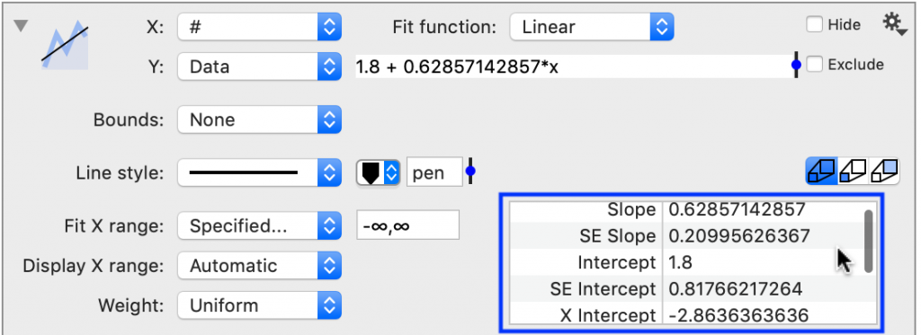
This is a scrollable list containing the fit parameters and goodness of fit results. You can highlight items in the list to copy the values.

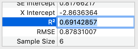
The number of digits shown is controlled by the same slider to the right of the fit equation.

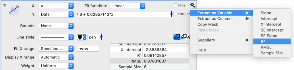
Extracting Results

Fit results can be extracted into global variables to be used in other equations.

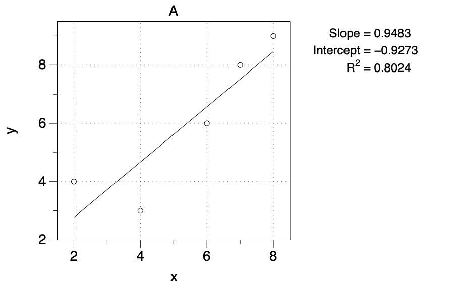
Displaying Results

Fit results can be shown in any command or title that has a text box, using a token. For example, here a Text command is used to display the fit parameters.

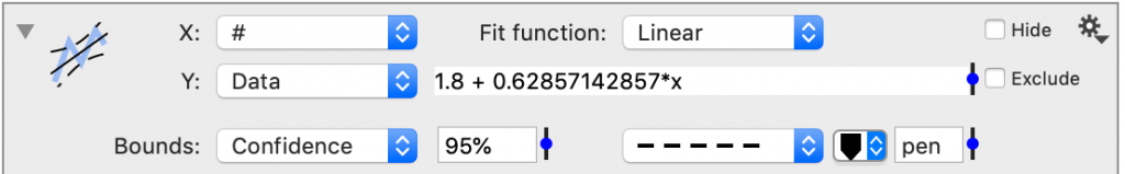
Bounds

The Linear fit has the option of displaying confidence intervals or prediction intervals.

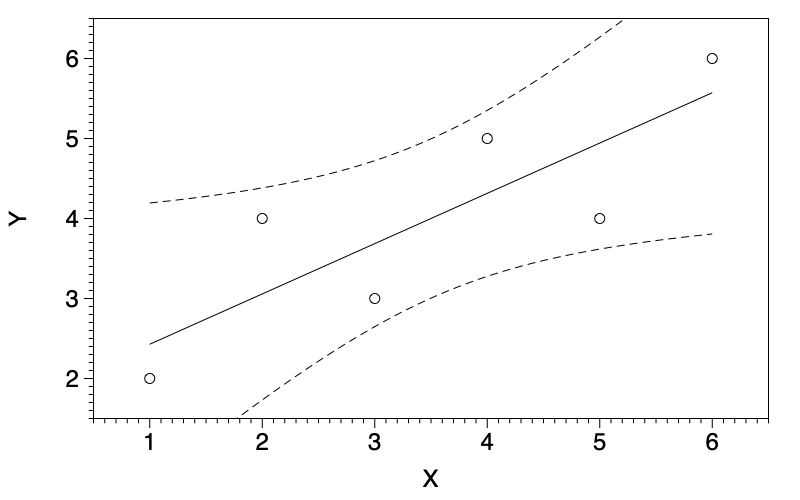
Line Style

Change the style, the color, and the width of the best-fit line.

The width of the line is set to the pen variable by default (value in pixels). To change, enter a number, a number variable, or a multiple of the pen variable.

Change the value of the pen in the Style settings.

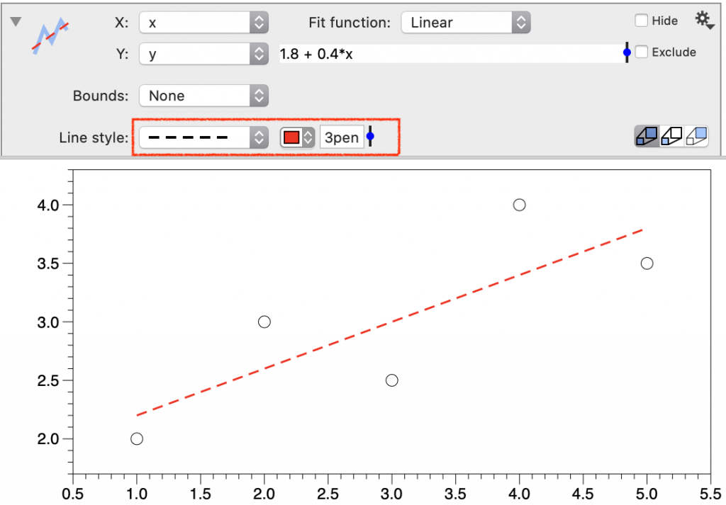
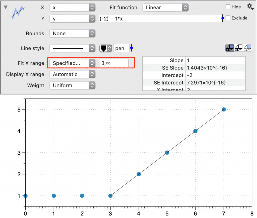
Fit X Range

Specify the range (lower, upper) of the X data included in the fit. This setting can affect the fit result.

• Everything (default) — Fit the entire range of input data.
• Specified — Enter the upper and the lower as comma-separated numbers or number variables.

For example, the range is set to ‘Everything’ by default.

Step 1: Change to Fit x Range to ‘Specified’. An entry box appears to the right. The upper and lower bound include the entire range. (-∞, ∞).

Step 2: Change one or both of the values.

Display X Range

Specify the range of the fit line that is drawn in the graph. This setting will not change the fit result.

• Everything (default) — Display the fit line corresponding to the range of input data.
• Include — Enter one or more numbers, or number variables, as a comma-separated list.
• Specified — Enter the lower and upper range of the fit line (i.e., lower, upper).

For example, select ‘Include’ and enter, ‘0’.

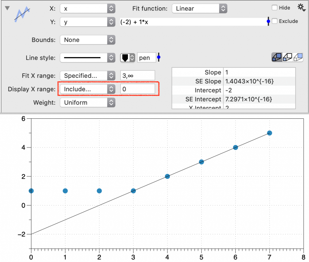
This extends the range of the displayed best-fit line to include 0.

Weight

Select a column to apply weight to particular data points.

Fill

You can apply a Fill to the graphing. The fill span from the fit line to the axis. When you have bounds displayed, the fill is applied between the bounds.

Residuals

At the very bottom of the command, there is an additional disclosure triangle to the left of the word Residuals. Use this to visualize the distribution of the residuals around the fit and to test the impact of outliers.

When you expand this section, you see the following, where the y-values are the residuals from the fit function versus x.

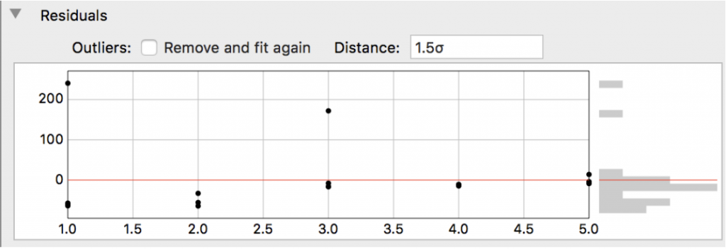
If you click the Outliers check-box a green line appears corresponding to 1.5*σ, where σ is the standard deviation of the residual. The points outside this green line are considered outliers according to this criteria.

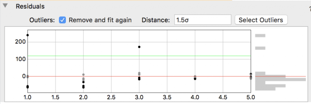
The fit is then recomputed with these points excluded from the fit. To identify the outliers in your data, click the ‘Select Outliers’ button in the right corner. Any outliers will then be highlighted in the Data Table.