Plot Action

Use the Plot Action column to perform mathematical actions on columns of data. Create the Plot action columns using the Other drop-down menu above the column definitions.

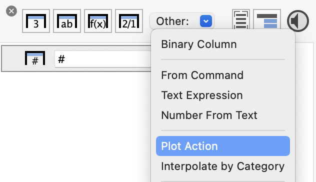
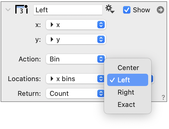
To use this action, the first step is to select the x and y input columns. The next step is to select the computational action from a menu, as shown in the following screen shot.

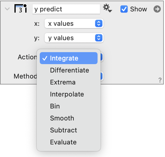
The entries below the Action menu change depending on what you select. The column returns a single column of numbers. In the following sections, each Action is explained further.

Integrate

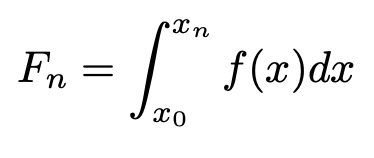
The Integrate action computes the accumulative integral. Specifically, for a particular row the value is the integral of the xy plot up to that row. As demonstrated below, there are three options for how the integral is calculated: Trapezoid, Left and Right.

Note that the first entry is always 0. For each interval, the integral changes by what is considered the integral for that interval. The first interval in the table is between 0 and 1 in the x direction. The y values are 1 and 2, so the trapezoid approximates the integral by computing width times the average of 1 and 2. The Left option uses the value at the starting point and multiples the width. The Right option uses the value at the ending point and multiples by the width.

The trapezoid method is more accurate when you have a smooth function, but the left and right options are useful when you want to use this method to compute an accumulative sum. In that case you would use the row column (#) as the x coordinate.

Differentiate

Computes the derivative at each x location. There are several ways to approximate the derivative.

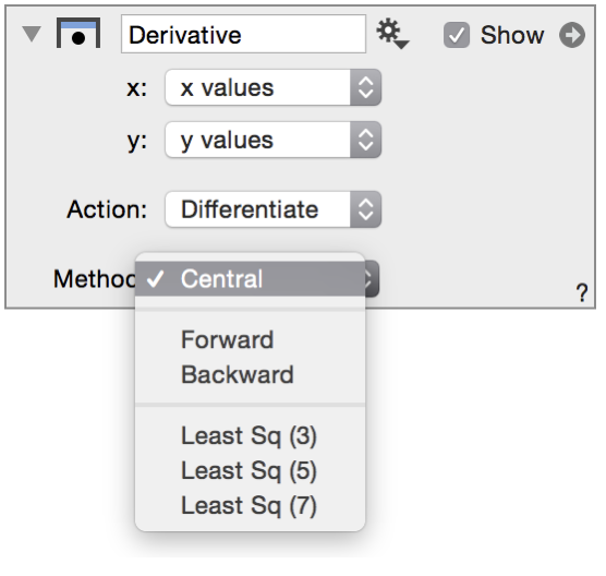
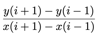
The central derivative approximation uses a second order polynomial through the current point and the point before and after and differentiates that approximation. If the x values are uniform it simplifies into what is typically called the central derivative approximation, namely for row i the derivative is computed by

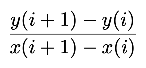
Forward and backward use one sided derivatives. They are less accurate for smooth functions. The Forward difference for row ‘i’ is computed by

The least square options are computationally a little bit more involved. They use three, five or seven neighboring rows (one, two or three before and after), compute a least squares linear fit to the (x,y) values at those points and then return the slope of that line.

Extrema

To find the overall maxima or minima for a column, you can use a Number from Column global variable; however, if you want to find local minima or maxima you can select the ‘Extrema’ option from the Action menu.

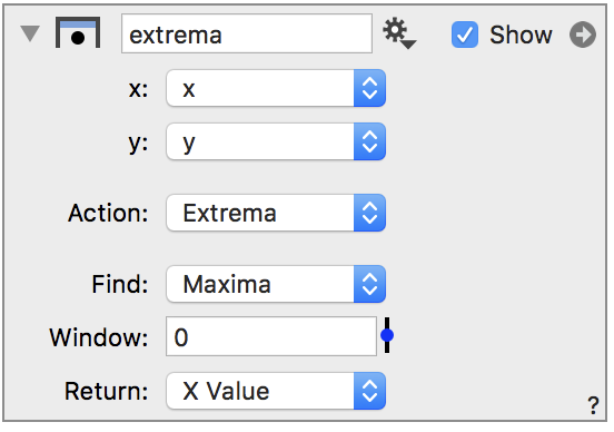
The output column has a non-empty row at the maxima, and you can choose to either return the x or y entry at that maxima. In this simple example, the x value is returned.

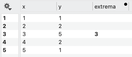
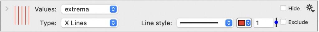
When the window is 0, the action finds every local maxima. A local maxima is defined as a row where the previous row is less than or equal, and the next row is strictly less. If the y column has a lot of noise you get a lot of local maxima as is shown in the next figure, where the lines are drawn over the data using a Lines command.

The graph is created by using the result from the Extrema action in a Lines command to draw the horizontal lines associated with each maximum.

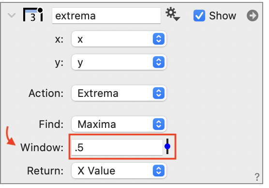
The Window setting can be used to specify a minimum distance between the extrema. In this case, the maximum has to be both a local maximum and no value within the given window can be larger. In the example, when the window is set to 0.5, the local maxima’s due to noise are removed, as shown below.

To show the minima and the maxima create two Plot Action columns, one for each. Here the y value is returned and two Points commands are added to show the location of each (i.e., the max and the min).

Interpolate

The Interpolate action allows you to use known data to approximate values at locations where the data is not known. For example, if you are given a sampling of a function at points x1,…,xn, you can approximate at points in between those values. There are multiple ways of interpolating between data points that typically involve approximating a function by fitting a line or polynomial through neighboring points. The function can then be used to approximate values at locations were there is no data.

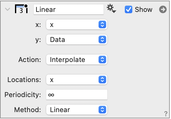
The Interpolate action allows you to choose between a number of different approximations methods as shown below.

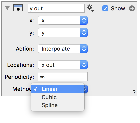
You select the x locations where you want to interpolate the x,y data sets as a column.

• The ‘Linear’ option means that the approximation uses the two closest points and approximates the function with a straight line between the points.
• The ‘Cubic’ option uses four points to fit a third degree polynomial through the points and evaluates that polynomial at the point.
• ‘Spline’ uses a cubic polynomial on each interval such that the second derivative is continuous across the interval. This is same as the spline option in the Plot command.

You can chose a different column for the locations or use the same x column for both when interpolating missing values.

Here is an example where the three interpolation methods are compared.

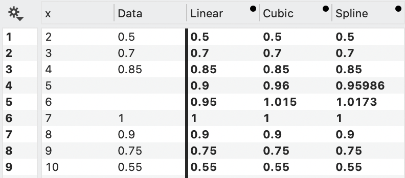
Here the points are interpolated using the linear approximation. The known points are in black and the interpolated points are open red circles.

Here is the same data interpolated with the cubic approximation.

Bin

In order to group data based on either numerical or categorical groups, DataGraph contains drawing commands such as a Histogram and the Pivot command. These drawing commands also allow you to extract the results of the binning; however, there may be some cases where you want to bin a set of data without plotting or you want to use non-uniform bin sizes. In these cases, the Bin action can be used to analyze data while specifying the bin locations directly.

You must have a column set to specify the locations of the bins and whether these locations define the Right, Left, or Center points of the bins. You can also select for an Exact match.

Here you can see the impact of choosing different options. This table shows the count for each bin. For the left option, the bin starts specified value and ends at the next bin, where the left location is included, e.g., [left,right).

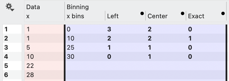
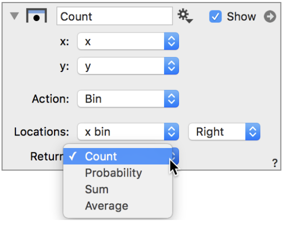
Other options return the Probability, Sum or Average for that bin.

Smooth

The Smooth action requires two columns (e.g., x,y), and generates a single column of data. Smoothing can be used to reduce noise in a data set as shown below.

There are three options available for data smoothing.

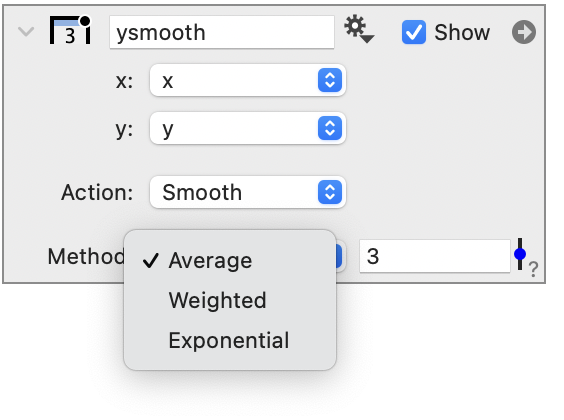
For a moving average, you specify how many previous values to use in the average. This functionality will ignore the x column and just look at the order for the y column. For the first column, it uses an ever larger average, so the first value is the same, the second value is the average of the first and second, the third is (y(1)+y(2)+y(3))/3. The fourth is the average (y(2)+y(3)+y(4))/3, etc.

For more information on these techniques, see: Wikipedia – Simple Moving Average.

Evaluate

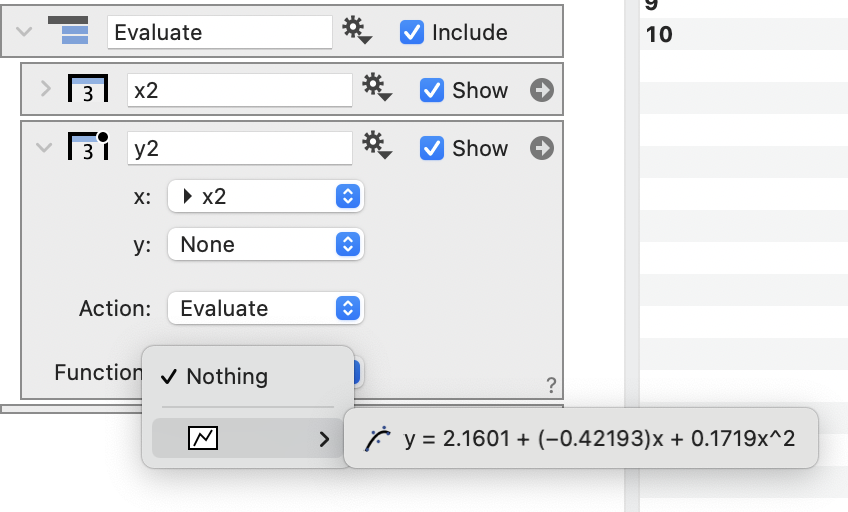
The Evaluate option allows you to evaluate a function, y=f(x), at discrete x locations. It required requires one column (x) and either a function from a Fit command or from a Function command.

Available functions will be shown in the Function drop-down menu.

Subtract

The Subtract option works very similar to the Evaluate option, but in this case you to subtract a function, y=f(x), from discrete y values. It required requires two columns (x,y) and either a function from a Fit command or from a Function command.

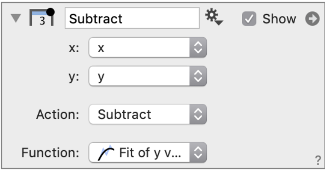
This column can be useful for calculating residuals from a function fit, since the residuals extracted from the Fit command directly will only provide residuals for the data used in the fit.