Multivariable Fit

The Multivariable Fit command finds the best-fit line for equations of the form

where y is the dependent or response variable and the x values are the independent or predictor variables.

Background

Simple linear regression is conducted in DataGraph using the Fit command, where y is a function of x (e.g., y = ax + b). The Fit command also can be used for exploring other functional forms where y = f(x), such as high-order polynomials, exponential fits, and LOESS.

To explore relationships where y is a function of more than one variable, such as multiple linear regression, use the Multivariable Fit command. That is you have a single dependent variable, Y, and multiple independent variables, x1, x2, …, xn.

Mathematically if y depends on two variables x1, x2 the dependence can be written as y = f(x1, x2). For example y = a*x1 + b*x2, or y = a0 + a1*x1 + a2*x2. The data values for (y,x1,x2) are given in a table and you need to find the values for a0,a1, and a2 that minimize the error (i.e., residuals).

The Multivariable Fit command minimizes the sum of the residuals as follows

Input

When a Multivariable fit command is added, the object looks as follows.

Consider a simple example where we want to fit y = f(x1,x2).

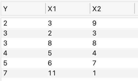
Select the dependent variable using the Y menu. Select the independent variables using the menus just below the Y menu. Click the plus buttons to the right of the x values to add independent variables.

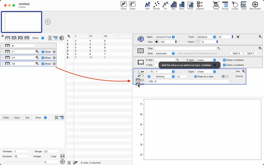
To more quickly populate the list of independent variables, drag and drop the column objects onto the command.

Type

By default, the fit Type is set to ‘Linear’.

The Type can also be used to set to ‘Scale’ or ‘Arbitrary’.

When the Type is ‘Scale’ the constant is set to zero. When Type is ‘Arbitrary’ a non-linear curve fitting algorithm is used to solve any function in the form y = f(x1, x2, …, xn) (i.e., Levenberg–Marquardt algorithm). If you choose ‘Arbitrary’, expand the command and enter the function as shown below.

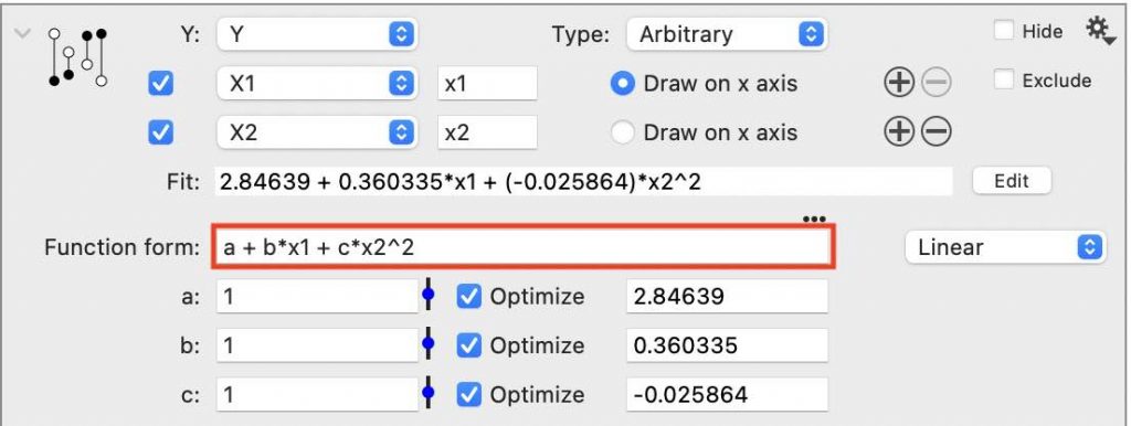
Below the Function form entry box, a list of unknowns is automatically populated with an initial guess set to 1 by default. Note that for non-linear curve fitting a good initial guess is important for the algorithm to converge.

For the Arbitrary fit option, you have the choice of minimizing y on a linear or logarithmic scale (menu option on the right of the Function form). For more information, see the discussion error in the Fit command documentation.

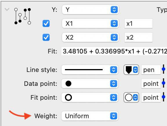
Weight

Select a column to apply weight to particular data points.

Output

Fit

The best-fit equation is below the input variables.

Use the checkboxes to the left of the input to exclude a variable from the fit. Note the impact of removing X2. The fit equation only includes X1.

Graph

Functions in the form of y = f(x) are two-dimensional problems and well suited to drawing in 2D space. Functions in the form of y = f(x1, x2, …, xn) are multidimensional dimensional problems that are impossible to draw in two dimensions. This inherently poses an issue for representing multivariable output in 2D space.

In DataGraph, you are given the option of choosing which independent variable (x) you want to plot along with the dependent variable (y).

In the graphical output, the input data and the fit results are both drawn. The line between them shows the magnitude of the residual. In this graph, the point with the highest residual is pointed out. When the two points overlap, the best-fit equation is doing a good job of predicting y at a given x.

If you toggle the Draw on x-axis button, the graph will change to show the Y values in terms of a different X value.

The x-axis label can be set up to change automatically by setting the X title to use a token.

Select the X-label token using the Axis settings, as shown below.

Table

Click the top left corner to expand the command to see the output in a table format.

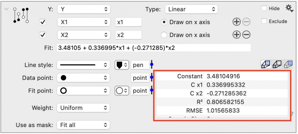
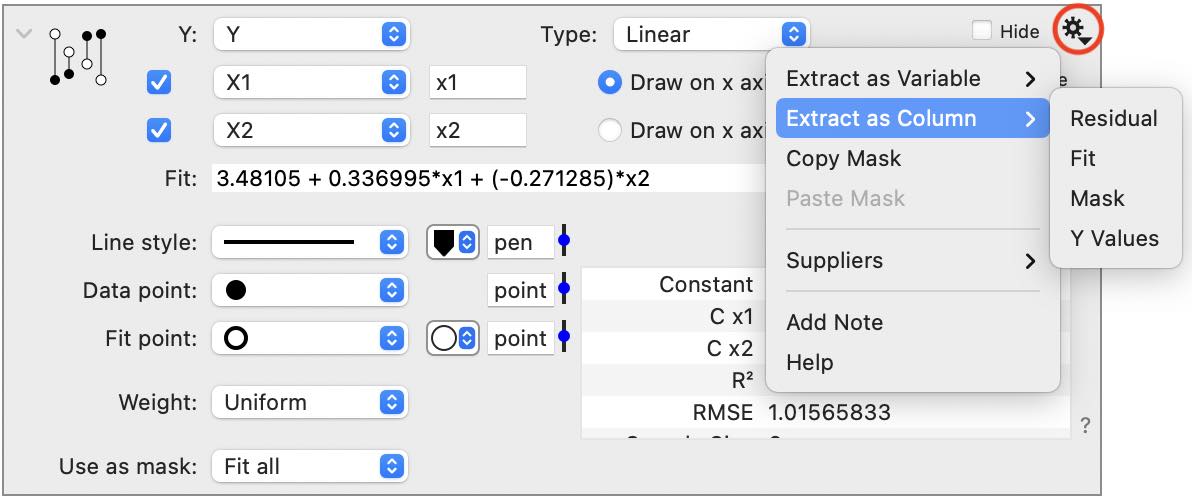
Click the gear menu to extract any of the values from the table as variables or columns for the residuals, fit, etc.