Table

A Table, sometimes called a data frame is a collection of columns and rows. The structure and limitations are as follows:

• The column names have to be unique (case sensitive) but can have spaces and Unicode characters.
• Each column has the same number of rows, but entries can be missing.
• The type can vary and there is a number of different types, not just numerical and text.
• The structure of the table, that is the name and type of each column is defined even if there is no data. This is similar to other data types like images and means that column names and types will show up in menus in the user interface even when nothing has been computed.
• When you have a time sequence of tables, every time value has the same structure.

Column types

• Number – numerical value.
• Date – encodes a calendar date. View this as a numerical value: the number of seconds since the reference date Jan 1st, 1970.
• Point in 2D – In expressions, you refer to the entries as .x and .y
• Point in 3D – In expressions, you refer to .x,.y,.z
• Path in 2D – a polygon for every row. Same restriction as the 2D Path variable.
• Surface in 3D – a triangulated surface in every row.
• Mask in 2D
• Mask in 3D

Creating a table

Use the table button in the gear menu to create a table from scratch. The main methods are

• From a file: Read in a text file, such as a comma or tab-separated file. You create an importer and define the structure. This is a very flexible method to import data and allows you to apply filters during the import.
• Using expressions: Use this to create a table from scratch. For example, if you want to evaluate a function at uniformly spaced points, create a table with random numbers, etc.

Modifying a table

You can not modify individual entries in a table easily. Use a program like DataGraph to do that. ImageTank is geared towards a computational pipeline where data comes from files or computation. You can modify entries programmatically, however, and use the gear menu for that.

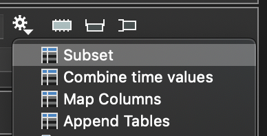
• Subset, which could be called a filter, extracts a subset of rows based on criteria. This creates a table with the same structure. Use this for example if you want to focus on rows/records where a given column is positive or inside/outside some interval.
• Combine time values: Variables in ImageTank can be collections, called time series. For example, if you have 100 files and create a table from each file using the table importer, if you want to concatenate all of these tables you are combining the time values.
• Map Columns: Allows you to map individual columns. For example, if you want to sum up columns, break a point column into an x column and a y column or combine two numerical columns into a single point column, etc.
• Append Tables: Combine tables from different variables with the same structure. The Combine action combines across time for a single variable, this combines tables from multiple variables.

Example: Use expressions

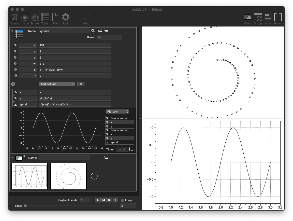
The most common column type is the numerical column. This is what you will use for an x-y plot for example. Take a simple example, and generate an x-y table from an expression. There are a number of concepts used in the following figure that are explained below.

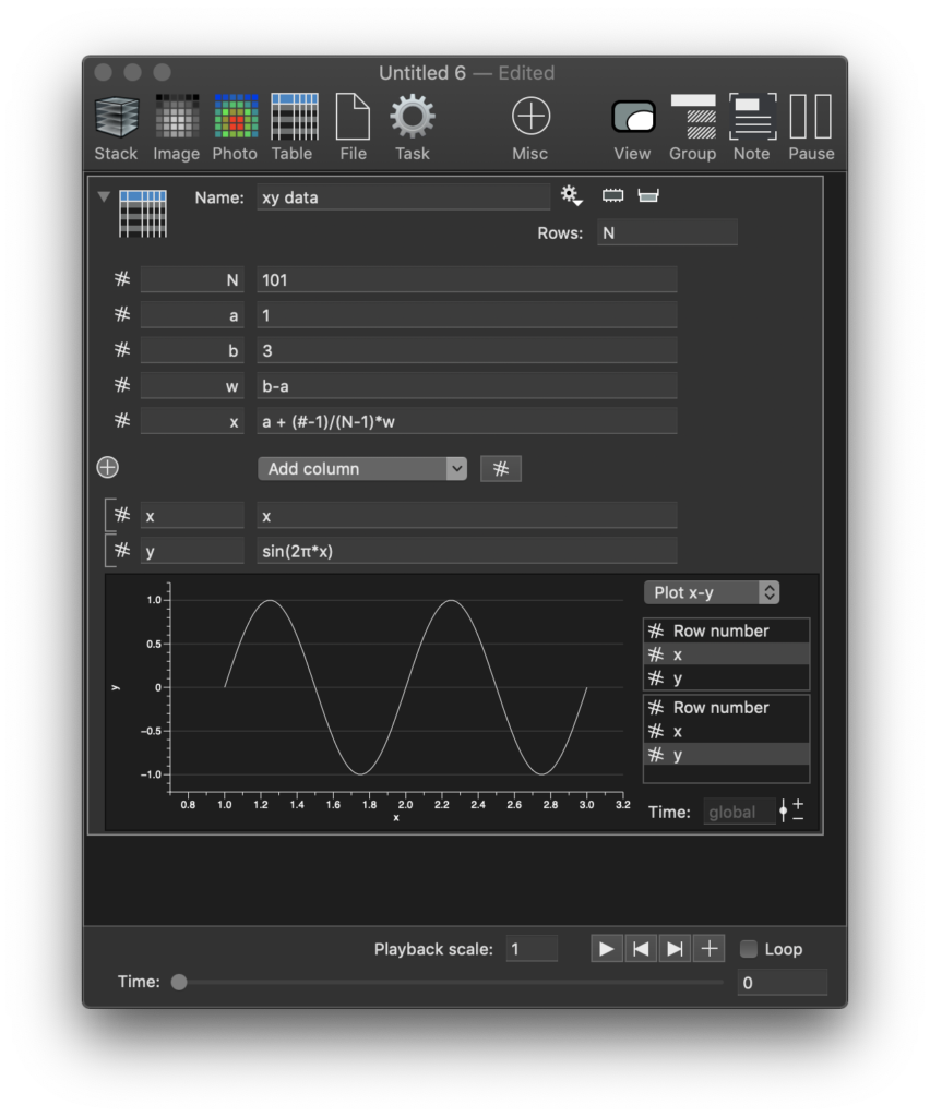
• The variables N, a, b, w, and x are local variables that are created using the small plus button that is to the left of the “Add column” menu.
• The top entry N is used to specify the number of rows. Since it is a local variable it can be used in any expression field inside the variable as well as subsequent local variables.
• a,b define the starting and end of the interval, and the w variable then refers to them. For local variables, you can use other local variables as long as they are defined above. The w variable is used to show that and to simplify the x variable a little bit.
• The x is a local variable, but local variables can vary based on the row number if they depend on the row number. The # variable is defined implicitly as a local variable and is essentially a column with length N. That makes x a variable and a column as well.
• Below the local variables are the column names and here we define two columns x and y. This is not a local variable. The reason you can use a function of x for the y column is that x is already a local variable. If you called the first column xcol you could not use xcol to define the second column.
• The variable monitor is switched to an x-y plot and the columns can be varied to quickly do an x-y graph.

Example: Draw an x-y graph

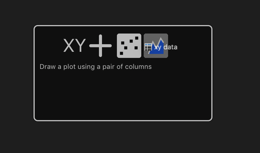
You can draw the content of a table in various graphing windows, xy, 2D, 3D, etc. The standard is the x-y plot. Increase the document window to reveal the drawing canvas and drag the table onto the right side. Since you have a numerical column it suggests two drawing commands, scatter, and line. Drag onto the line command

This creates a new xy graph and adds a single command. Currently, this is relatively limited compared to DataGraph, but that will be fleshed out based on requests. In fact in order for this window to work you need DataGraph to be licensed on the machine. You can recognize the style, canvas, and axis commands and they are sub-sets of what DataGraph has.

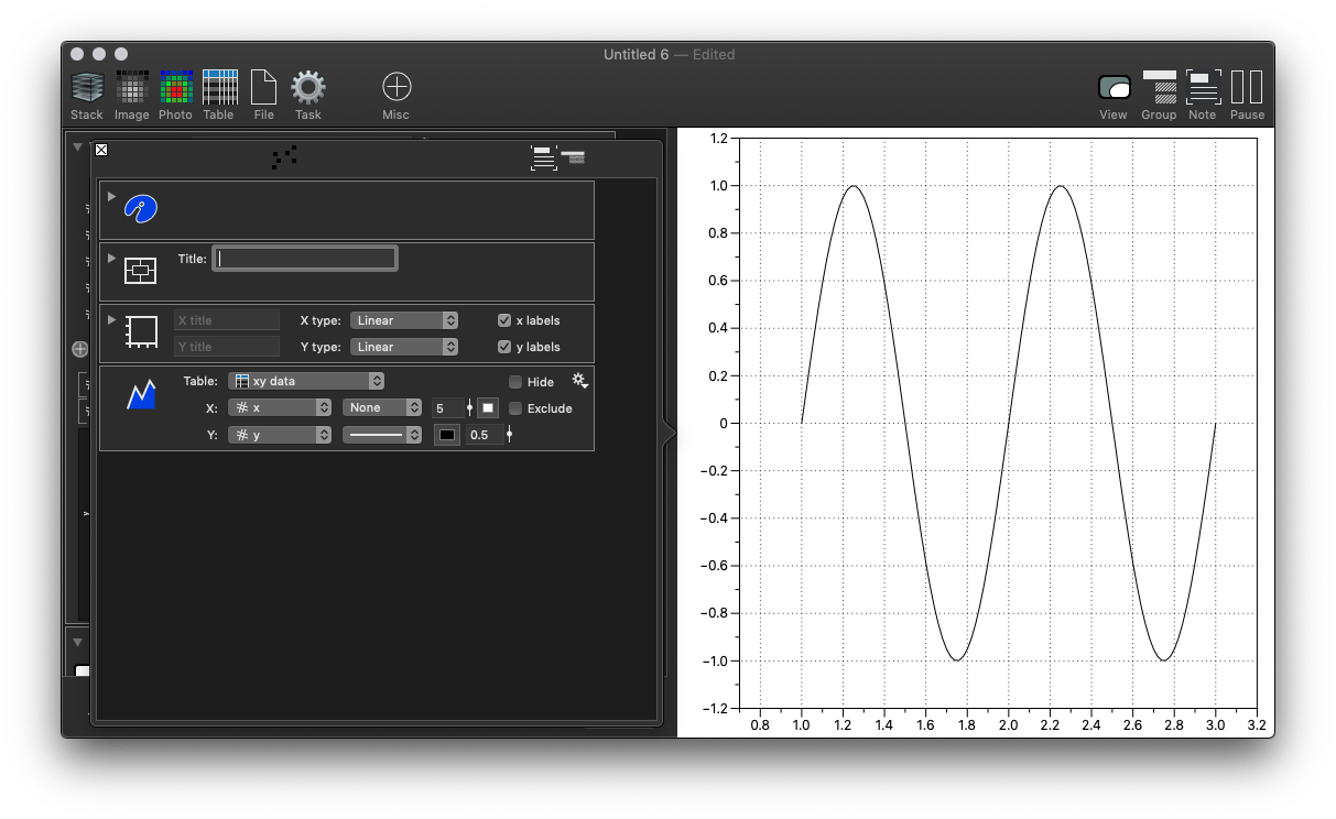
One big contrast with DataGraph is that

Example: Draw in 2D

XY graphs are two-dimensional graphics, but the x and y axis is independent so it is not very good to use them for data where the x and y values are really spatial coordinates and you want the scale to be the same in x and y. This is what the 2D space drawing handles. It was not an option in the previous example because there wasn’t a 2D point column. So let us add that to the above table. Add a 2D Point using the “Add column” menu for the table. Use an expression with two components to define the point value for each row. When you drag the table onto an empty drawing region you get the xy option as above but also a 2D option with a scatter option. The expression is “r*(cos(2π*x), sin(2π*y))” where r is a local variable defined as x, but you could use x instead and avoid the local variable.

Example: Mapping a table

If you have a table that has a 2D Point column but you want to draw the components you need to extract the x and y components into columns in order to draw them in an x-y graph. This is done by going to the gear menu for the variable and selecting the “Map Columns” option.

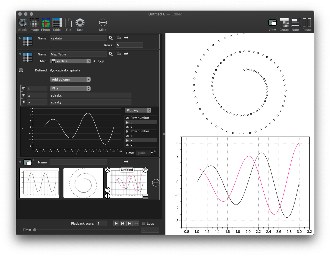
• The x column is copied, and if you have column types that are not a number or point this is how you carry them over to the new table.
• The x and y columns come from the spiral column in the source image. At the top you see a “Defined:” list that shows the numerical values that are defined as local variables. No additional local variables are defined here, but they could. The x is then simply ‘spiral.x’, the x component of the spiral entry. This is evaluated for every row.

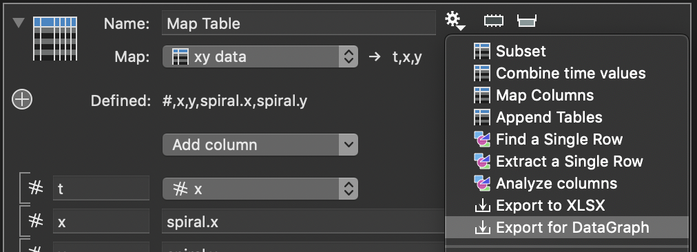
Sending data to DataGraph

DataGraph will not be replaced by ImageTank. See this write-up that addresses the difference between the programs. It is easy to send data from ImageTank to DataGraph. Since DataGraph looks at all data as a table, you do that by sending a table over. This uses the same mechanism as the CRAN package to save a data frame into a file that DataGraph can easily import.

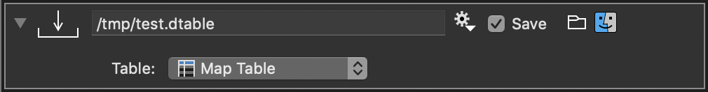
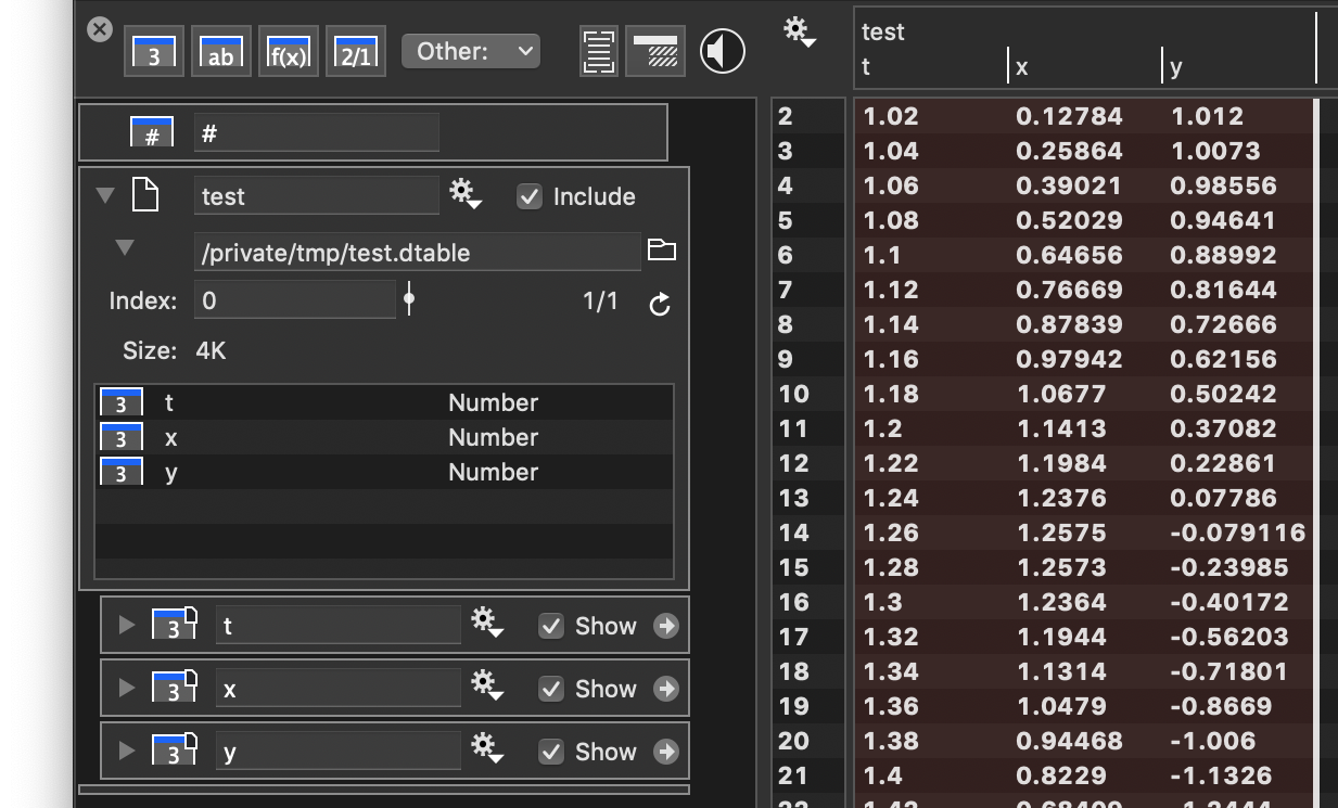
The first step is to export the ImageTank file into a ‘dtable’ file

What you get is a single object to save into a file. Just type in the name of this file, ending in ‘.dtable’.

Once you have this file, just drag and drop it into the column list in DataGraph

If you keep the Save checkbox checked, every time the data changes the file is resaved. Once it is resaved DataGraph will detect that it was updated and reload it. That will trigger any derivated content such as graphics to be updated.

The file will stay even if the ImageTank file closes, but if you use the /tmp folder it will be removed automatically by the system when it reboots or decides to clean up old files. That is the temporary folder after all. For that, you should save the file somewhere more permanent. Note that it might not be suitable to save it in a location that DropBox or other syncing utilities are trying to keep synced because the file might be written very frequently when you change values.