Newtons method in 2D
Summary
This is a little bit more involved example than the previous examples. This shows an example where ImageTank performs built in calculations to come supporting graphics, draws something rather than just using the monitor or DataGraph and allows you to interact with the graphic and not just type in the values to specify the input.
Mathematical component
This solves two equations with two unknown. It is set up as a vector valued function F(x) where x is a point in two dimensions and F has two components. That means that F(x) = 0 means that both functions have to be zero at the same time. The example functions are sin(x+y^2)=0 and x*cos(x*y) = 2. Not physically relevant, but give interesting graphics and a lot of solutions.
For a function of one argument, you can use Newtons method if you have an initial guess x_0 and then iterate using x_{n+1} = x_n – f(x_n)/f'(x_n). This extends to multiple dimensions, see for example wikipedia and scroll down to the nonlinear systems of equations part. The short answer is that the iteration involves solving a matrix equation

Where F is a vectored valued function

And the derivative is the matrix of partial derivatives with respect to x and y. The rows correspond to the function and the column correspond to the partials with respect to x and y

Visualizing the solution
Before we compute the solution numerically, we can sketch it up. This gives you a visual representation of the solution, but this visualization won’t give you the solution to more than a couple of digits. This solution will however be a good way to make sure that the numerical method works and see how the numerical solution depends on input parameters.
The first part is to visualize what the functions sin(x+y^2) and x*cos(xy)-2 even look like. These are functions that are defined in all of space.
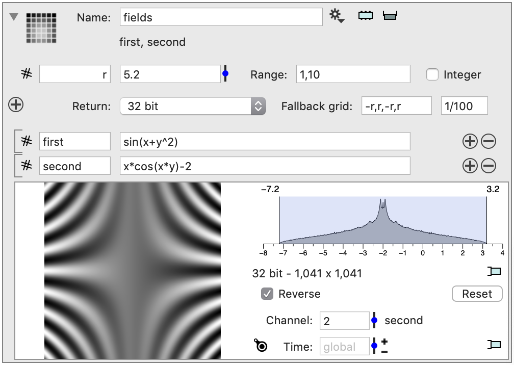
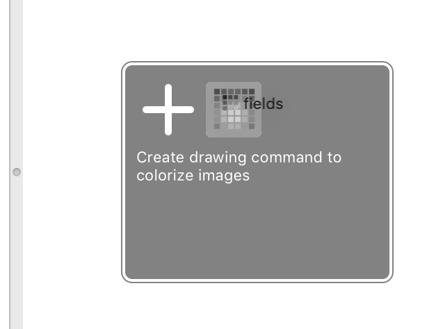
We use the Image variable for this. Images typically have multiple channels, such as red, green, blue for RGB pictures, or for microscopy intensity, and various flouresence markers. We use that here to create a channel for each function. To do that, first create the image
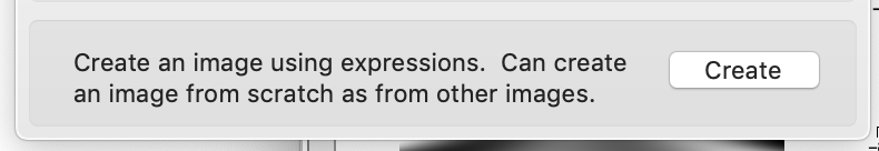
This action is typically used to compute fields based on one or more images, but since we don’t use an input image we need to specify the region and step size.
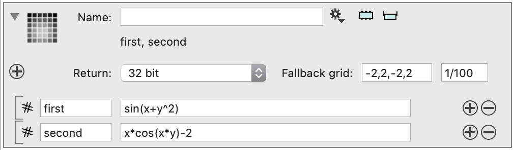
To experiment later, and to show how to add parameters into an expression click on the + icon on the left side.
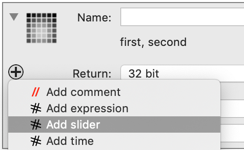
Give it a name (e.g. r) and range. Click on the small slider icon to the right of the variable to change the value using a slider. Then you can use r in later fields. This is used in the fallback grid settings. You can use the variable also in the expression that is used to define the field. Note that x and y are implicitly defined to be the grid location. Click on the monitor entry to preview the image.
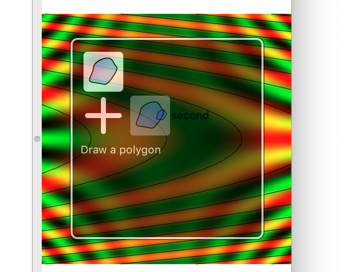
We want to get a visual representation of where each component is 0. This is what the thresholded path, sometimes called contour or level set is useful.
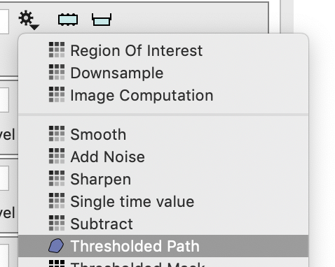
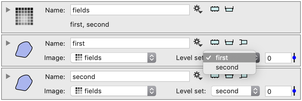
Create two such paths, and select different channels. Note that initially the level set value is not specified. Set it to 0.
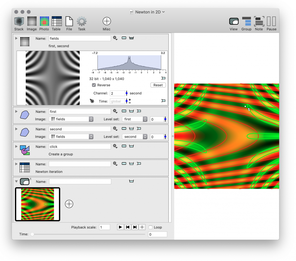
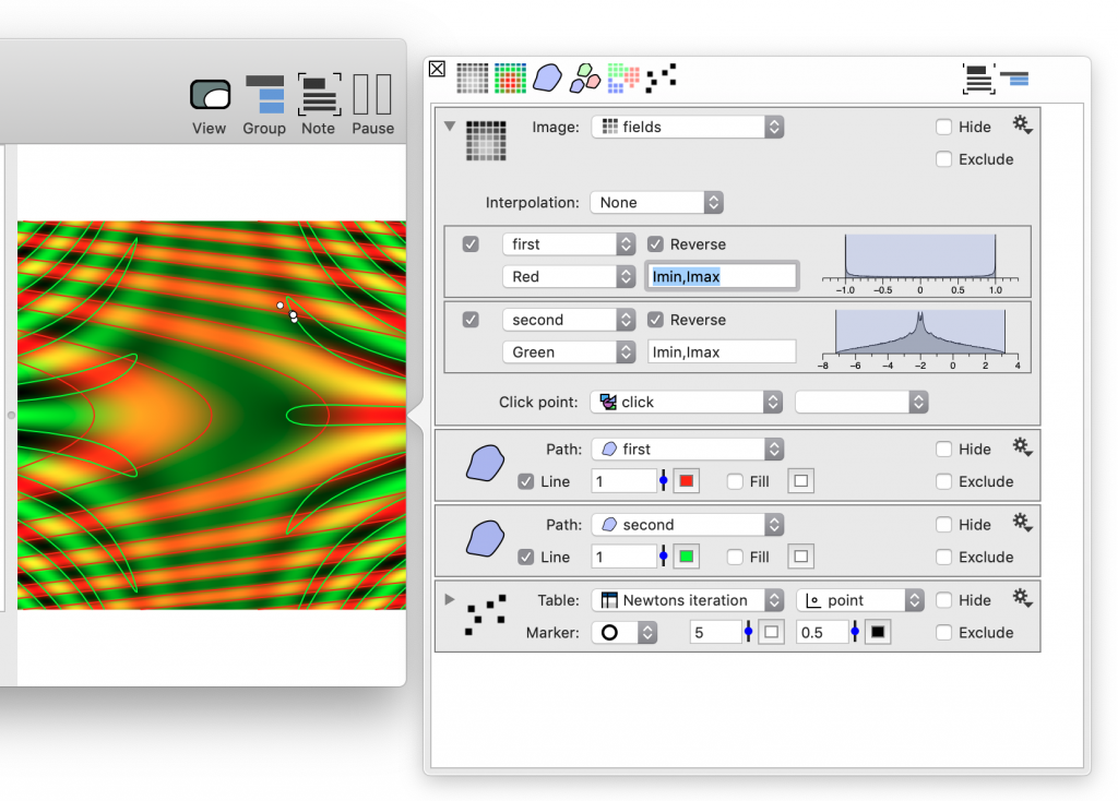
Next step is to draw this field. If you widen the ImageTank view you see a vertical bar. Drag the image (click on the icon and drag it) over to the white region on the right hand side.
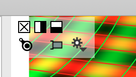
Drag the icon onto the image icon and release the mouse. This creates a drawing entry and adds that to the variable list. It has a default selection, but that typically needs to be tweaked to get the look you want. Here it is pretty simple. If you go to the top left corner of the graphic, you get an overlay with a few buttons. That has a side bar popup icon. Click on that to see the commands behind the drawing.
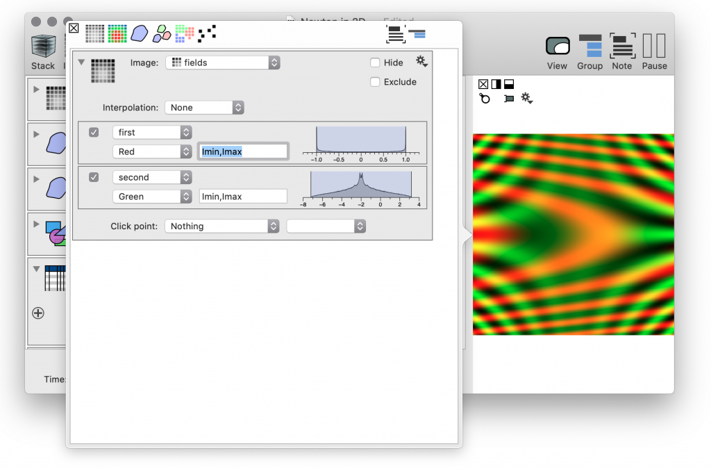
You can select the color for each channel and using either the numerical field or the histogram to the right of the color selector you can adjust the coloring range.
Now drag the two paths onto the same graphic. For the second path you have an option of changing the selection for an existing drawing command or add a new one.
Adjust the color and line style for the polygon. You can pop up the command list for the drawing at any time by going into the top left corner of the drawing and click on the side bar icon. Click on the color tile to see the standard system level color selector.
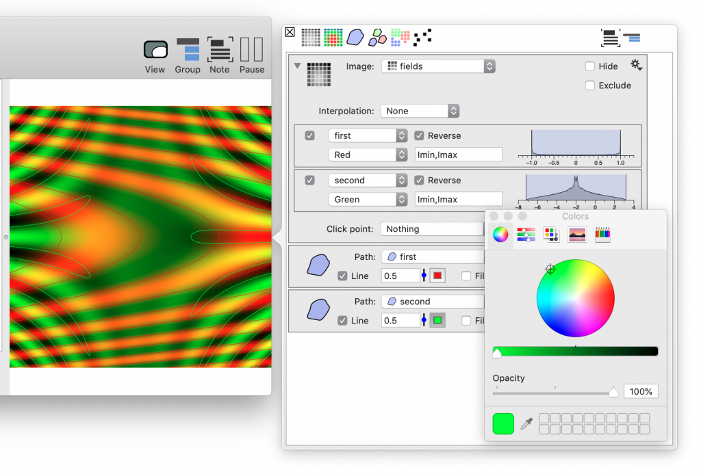
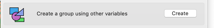
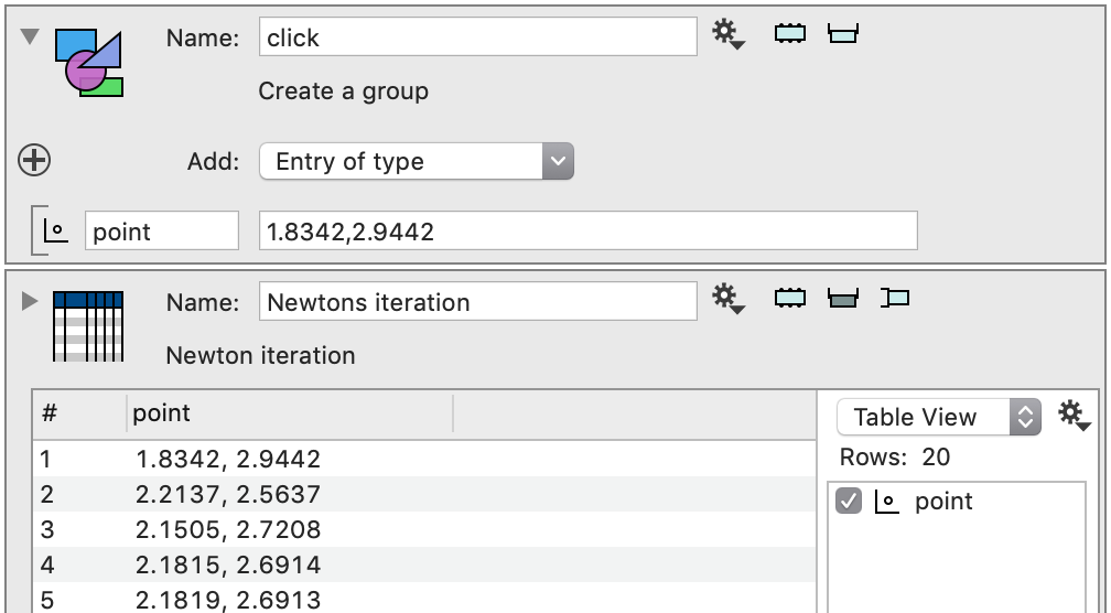
Each curve shows you where the function is zero. Where these curves intersect both functions are zero, and these are the roots of the vector valued system. We do this using Newtons method and implement a C++ function to perform the calculation. The numerical method will require a starting point and to make it easy to change this we are going to set things up so that we can click on the graphic we just created to specify the point. This action has two parts, we need a variable for the point and need to set things so that a click in the image will change that point. To start, create a group variable (Misc menu)
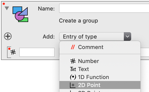
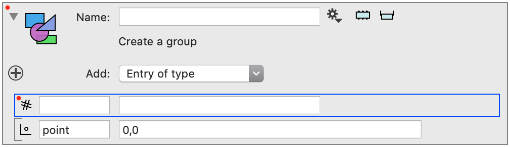
We need to add a point variable
To delete the default entry, click on the icon to select the variable. You will see a blue border around the entry, then hit the delete key. At this point the small red dot in the top left will go away.
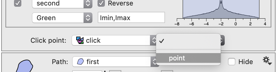
Once you have this, go to the drawing command for the image. One of the entries here is to specify what happens when you click on a point in the image. Select the group from there and then select the point that you want to change. When this is selected, when you click on a point in the image this click is used to set the selected entry in the group to this point.
Xcode Project / C++ Code
Create the external project and set the output table to return a 2D Point column.
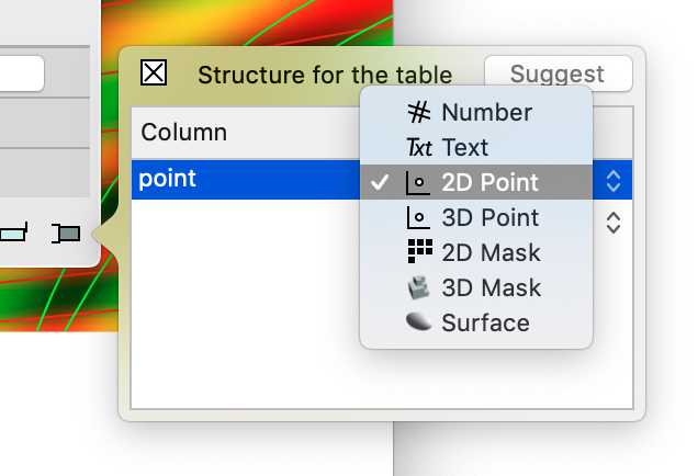
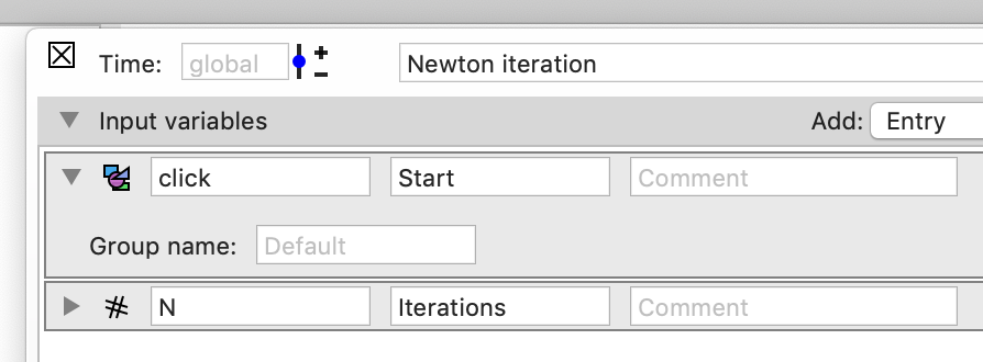
For the input, drag the group you just created into the input variable list and add a number. For the group variable you can specify the name of the structure. You can use the default name here. Make sure that the N variable is specified as an integer.
Create the Xcode project and paste in the following C++ code
#include "computation.h"

 DTTable Newton(const InputGroup &click,int N)
 {
     // Function is (sin(x+y^2),x*cos(x*y)-2)
     // Derivative of F is a 2x2 matrix
     // [cos(x+y^2)              cos(x+y^2)*2*y ]
     // [cos(x*y)-x*y*sin(x*y)   -x^2*sin(x*y)  ]

     // F(x) = F(xn + (x-xn)) approx H(x) = F(xn) + DF(xn)(x-xn)
     // Instead of F(x) = 0, find H(x) = 0
     // Iteration is
     // x_(n+1) = x_n - (DF(x_n)^(-1))*F(x_n),

     double x = click.point.x;
     double y = click.point.y;

     DTMutableDoubleArray pointList(2,N);

     double ux,uy,vx,vy,det,j11,j12,j21,j22,fx,fy,sx,sy;
     for (int i=0;i<N;i++) {
         pointList(0,i) = x;
         pointList(1,i) = y;

         ux = cos(x+y*y);             uy = cos(x+y*y)*2*y;
         vx = cos(x*y)-x*y*sin(x*y);  vy = -x*x*sin(x*y);

         // Compute the inverse of the Jacobian
         det = ux*vy-vx*uy;
         j11 =  vy/det;  j12 = -uy/det;
         j21 = -vx/det;  j22 =  ux/det;

         // Evaluate F(x)
         fx = sin(x+y*y);
         fy = x*cos(x*y)-2;

         // Step is J^{-1}*F(x)
         sx = (j11*fx + j12*fy);
         sy = (j21*fx + j22*fy);

         // Move the point
         x -= sx;
         y -= sy;
     }

     DTMutableList<DTTableColumn> list(1);
     DTPointCollection2D pointCol(pointList);
     list(0) = CreateTableColumn("point",pointCol);

     return DTTable(list);
 }
Some comments on this code
- Note that the name of the function is “Newton” and not the default name “Computation”. You need to change that in ImageTank or you will have problems when linking the program.
- DTMutableDoubleArray pointList(2,N) gives you a 2xN array which you can access as (i,j) i=0 or 1, j = 0,…,N-1. If you access out of bounds you get an error message. To catch those errors in the debugger, set a breakpoint in DTError.cpp
- DTPointCollection2D pointCol(pointList) views the list as a point collection. This will print an error message if the dimension is not valid. Because of how DTSource handles memory allocation, the pointList array is not copied but shared. In this code it doesn’t matter since we aren’t changing the values, but that also means that I could have created the pointCol object before I set the pointList values.
- CreateTableColumn(“point”,pointCol), the function CreateTableColumn is overloaded quite extensively to create different column types. Note that in other example codes this function name was used to create a number column but here it is used to create a point column which has a different type. This is because C++ treats these functions as different functions because the argument list is different. If you didn’t take the step of creating a DTPointCollection2D and hand that into the array, but instead handed the pointList directly the call CreateTableColumn(“point”,pointList) would be interpreted to create a number column and fail since the dimension is not valid.
Compile the code, hit the reload button if needed, and when you click on the monitor button you should see something like this:
Draw the points
Final step for the drawing is to draw it in the figure. To do that, drag the table over the graphic and drop it on the Point icon that pops up. The table and point column are automatically selected, but you can change the selection at any point.
Change things interactively
Now we can use this code to explore how well Newtons method works. A few observation you should be able to make
- When you click close to an intersection point you converge to that point.
- When you go further away what typically happens is that the first application of Newtons method can go pretty far away from where you clicked. Where it lands is somewhat random so it might continue bouncing around. Eventually it will land close to a solution and converge to it.
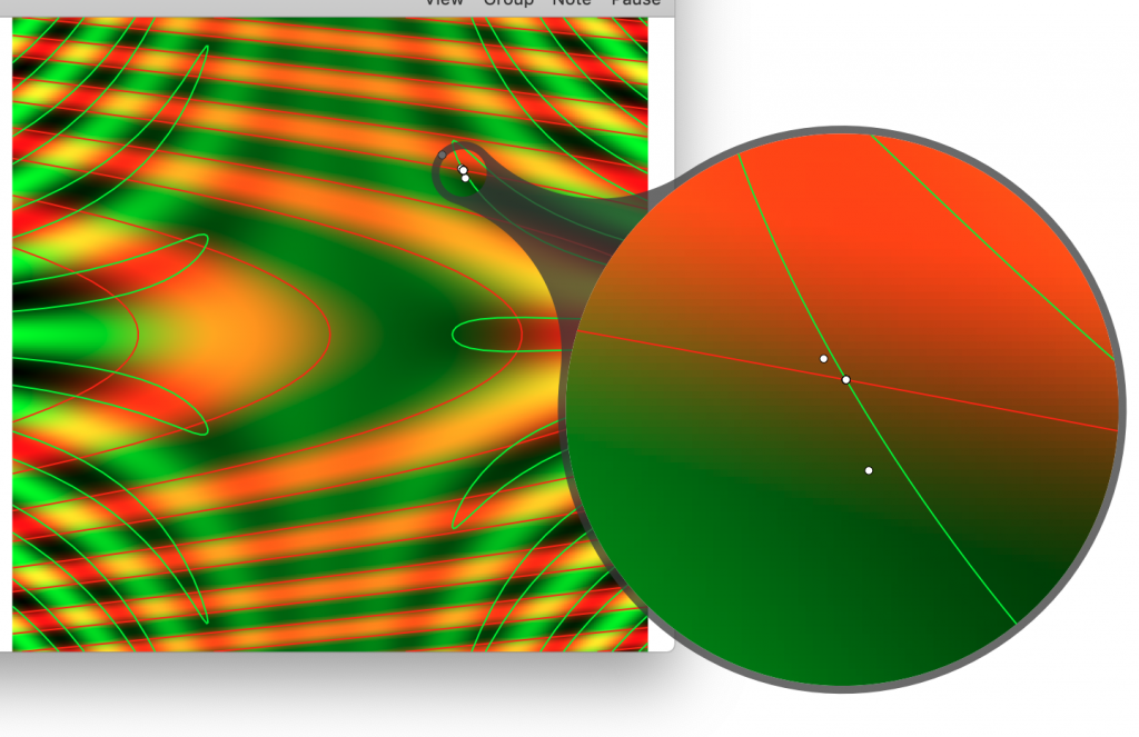
Loupe Tool
The Loupe tool can be very useful to zoom in on a detail without changing the graphic. You toggle it on and off by going to the top left corner of the graphic.
You can increase and decrease the size of the magnified portion by pinch to zoom action on your trackpad. If you hold down the control key and pinch the region that is magnified is changed. The points stay the same size, which allows you to see the detail.