Fixed Point Iteration

Summary

Numerical methods often involve an iterative process that converges to the solution. Newton’s method converges to a root of a function and it does that by creating an iterative process xNew = xOld – f(xOld)/f'(xOld). That is xNew = g(xOld) where g is an analytical function. In this example we go through a simple visualization method for fixed point iteration, and show how Newton’s method as well as more general functions behave. This example also shows how to use DataGraph to visualize the result and not just ImageTank. Since DataGraph has a lot of drawing power and is geared towards more interactive graphics you get the best of both by setting up an external program in ImageTank, that sends the data over to DataGraph that then can view the data. When you change the input in ImageTank, DataGraph will automatically update the graphic.

Setting up the program

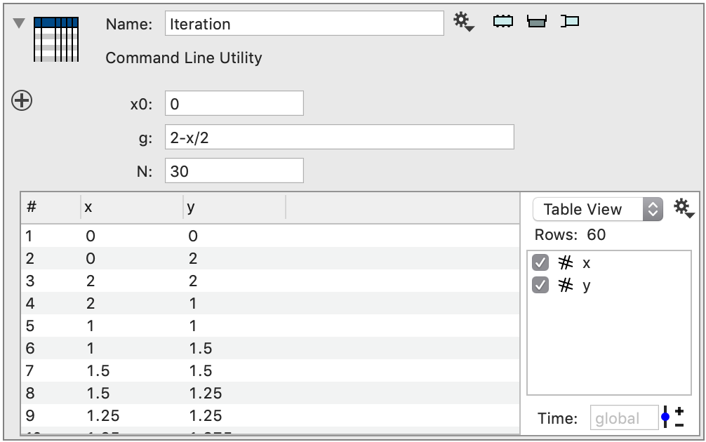
Use the simple group or Newton’s articles to see more details about how to create the Xcode project. You set up three inputs, the starting point, the function and how many iterations to create.

C++ Source Code

The purpose is to compute x_(n+1) = g(x_n), but for visualization purposes we save twice two columns and repeat each value twice in each column. Why this is done will be clear when you draw the result in DataGraph.

DTTable Computation(double x0,const DTFunction1D &g,double N)
 {
     DTMutableDoubleArray xList(2*N), yList(2*N);
     double gx;
     double x = x0;
     for (int i=0;i<N;i++) {
         gx = g(x);
         xList(2*i) = x;
         yList(2*i) = x;
         xList(2*i+1) = x;
         yList(2*i+1) = gx;
         x = gx;
     }
     
     DTMutableList<DTTableColumn> columns(2);
     columns(0) = CreateTableColumn("x", xList);
     columns(1) = CreateTableColumn("y", yList);
 
     return DTTable(columns);
 }

Looking at the result in ImageTank

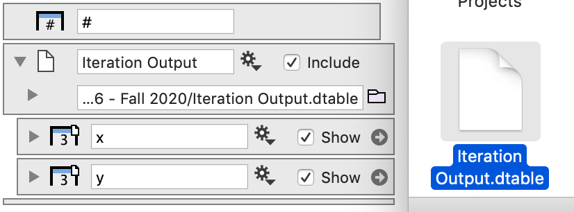
If you look at the result in ImageTank see the two columns and see how the values are repeated and shifted.

Sending the data to DataGraph

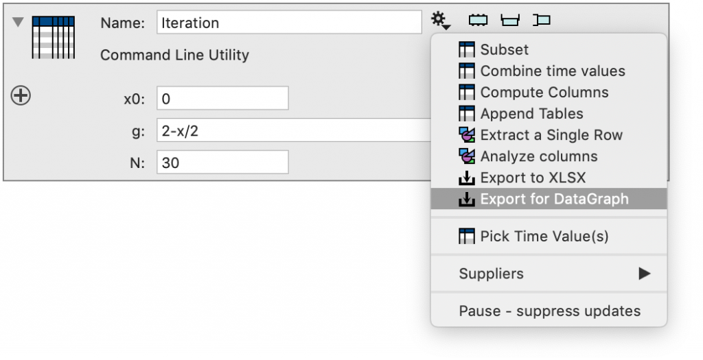
This creates an output entry. It doesn’t have a name, since it can’t be selected by any other variable. Instead you specify the output file name. You can click on the small folder icon to get a standard file dialog, or just type in the name of the file. If you use the second approach, make sure that the ending is .dtable

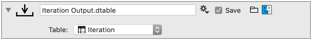
Click on the small Finder icon, and then drag the file into the column list in DataGraph. This creates a group in DataGraph and creates a column reference for every column that DataGraph can use. That means that number, text and date columns will be understood, but other column types will be ignored. Note that this requires DataGraph beta (4.6) Click to download the beta.

When the Save check box is selected ImageTank will save the file every time the data changes, and if DataGraph has a group that connects to this file DataGraph will reload the file. In that way ImageTank and DataGraph are connected, but ImageTank does not know if DataGraph is listening and DataGraph does not know that it is ImageTank that is re-writing the file. That file could be for example be written by R using the DataGraph package that you can download from CRAN.

Viewing the data in DataGraph

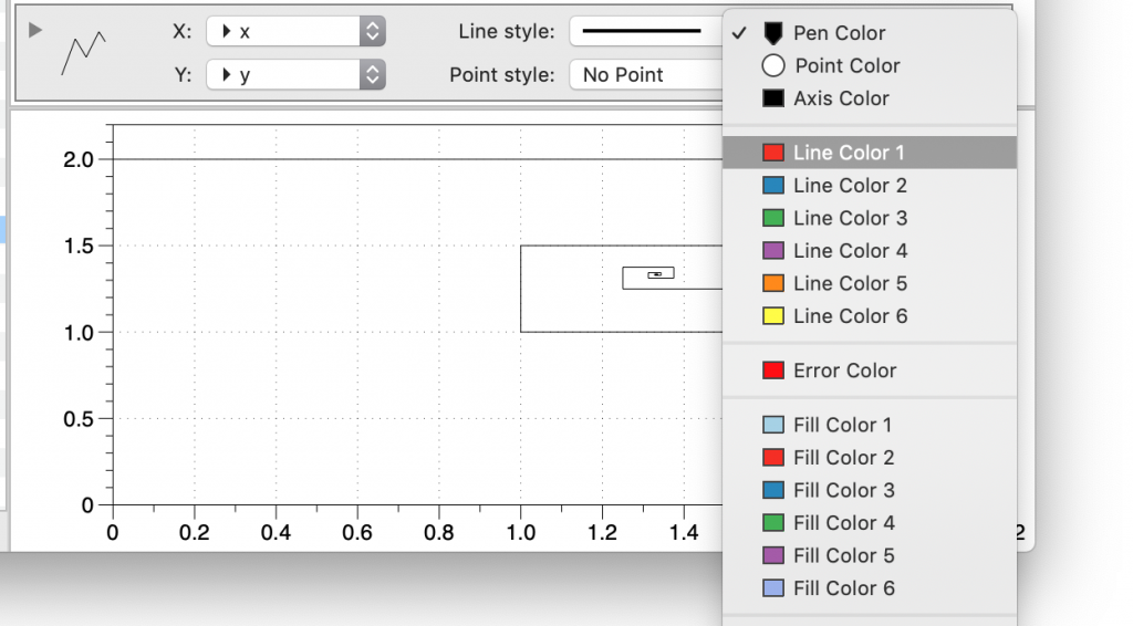
Once you have this data in DataGraph, select the two columns in the data table and click on the plot icon in the toolbar in the top left corner. This creates a Plot drawing command in DataGraph and selects the two columns. If you didn’t select the columns before you clicked the command you can select the colums using the menu. The iteration point were repeated the way they were so that you would get lines with constant x or constant y that connect the iteration points.

Now use the Function command (also in the Toolbar) to add two analytical functions, g(x) and y=x. Note that you need to specify the range of x for both of those functions, the default range is 0,1 which is too small.

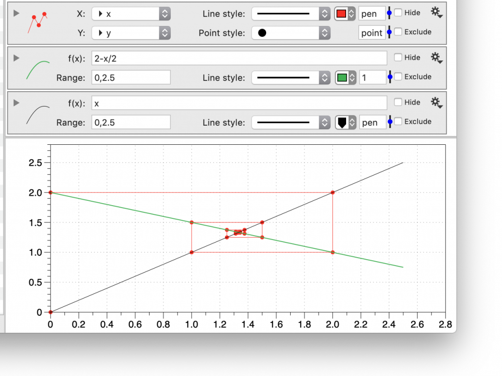
The intersection of y=g(x) and y=x means that x = g(x) so this is a fixed point for the iteration.

Back in ImageTank

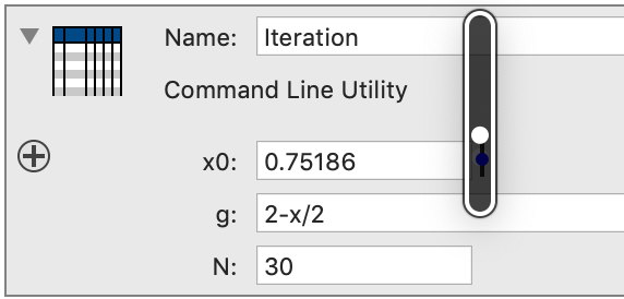
Start by setting up the input variable so that it can be changed using a slider. That is done by opening the side bar for the external program and in the detailed setting for the variable set the range. This will cause a small bar to show up to the right of the numerical field.

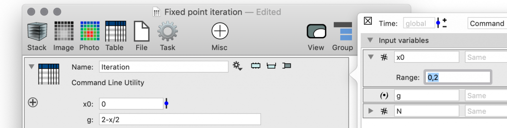
When you click on this button you get a pop-up slider that you can change. When you drag this around the value will change and the change is propaged through the entries in ImageTank that depend on this table.

What happens is that the output entry will get a message that the input changed. As soon as it is possible for this entry to do so, it will launch a background thread that computes the table and saves it to disk. This background thread will cause the external program to be executed. The table is then saved into the output file. When it is saved, DataGraph will notice that the file has been updated and reload the content. The lag time is only a fraction of a second. ImageTank does not know about this, so likely ImageTank is already computing a new value when DataGraph is drawing the previous one.

Change the function

This function is kind of boring, but the iteration does converge. The mathematical reason for that is that the error shrinks by about g'(c) where c is the fixed point. Since the derivative in this case is -1/2 that means that the iteration gets half as close to the fixed point x=4/3.

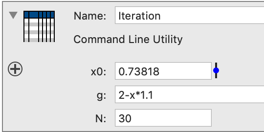
Now change the function ever so slightly, say to g(x) = 2-1.1*x. That needs to be changed in two places, in ImageTank specify a different function

And in DataGraph type in the same function

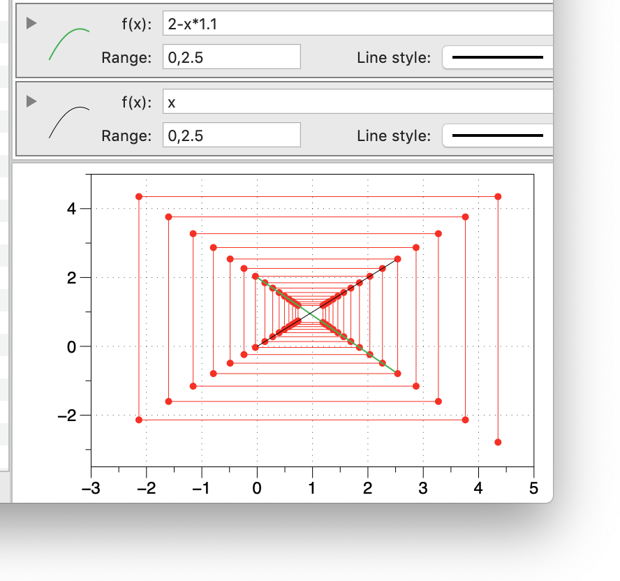
This diverges because g'(c) = 1.1 and the fixed point is when 2-x*1.1 = x so 2 = x*2.1 or x = 2/2.1.

Newtons iteration

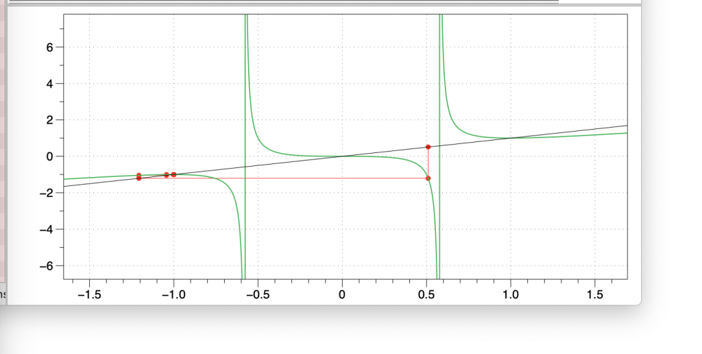
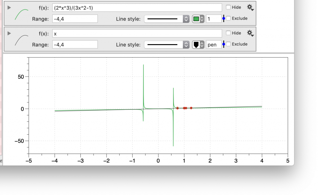
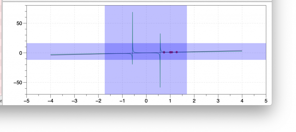
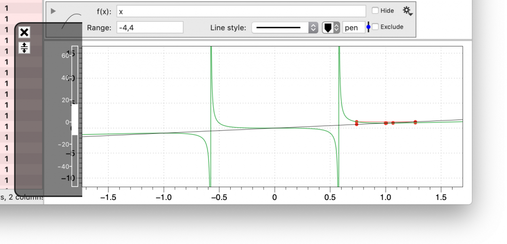
Newtons method finds a root of a function by setting up a fixed point iteration. The fixed point iteration applied the above functions will lead to a function that converges in one iteration so that is not very helpful, so instead use it to find roots of the function f(x) = x^3-x that has three roots, -1,0,1. The method is g(x) = x – f(x)/f'(x) which in this case is x-(x^3-x)/(3x^2-1) so g(x) = (2*x^3)/(3x^2-1). Change the g function in the same two places as before and you get a very different graphic. Note that I set the x range to -4,4 to capture the roots.

To zoom in, click on the graph and drag the mouse to start a cropping region. Note that if you just drag horizontally you only get one of those regions to show up, you need to also move vertically to get the other one. Start for example at the lower left corner of the region and move to the right and up. Once you get a reasonable region release the mouse

You can zoom in closer by either repeating the cropping action or move the mouse over the x or y axis and change the small white region with the mouse

You can zoom in without changing the range by using the Loupe tool from the toolbar. There is a shortcut Command-Shift-M to toggle this on and off.

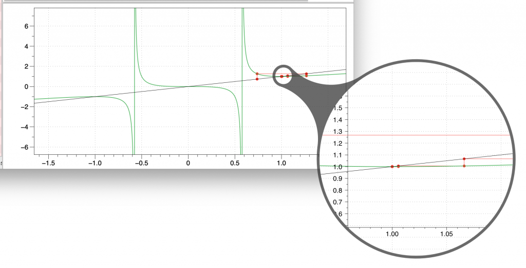
Now when you vary the initial guess you see how the iteration will not necessarily go to the closest fixed point.