Surface Intersection
An interesting example is computing implicit surfaces and intersecting them.
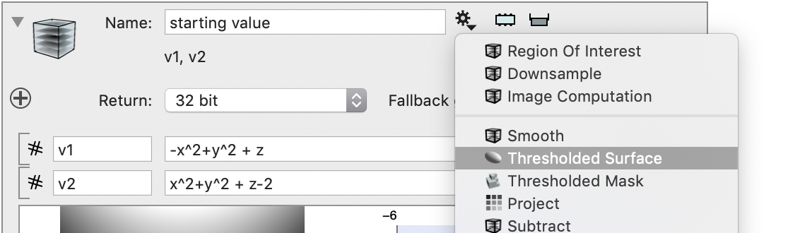
Set up two surfaces, defined implicitly by
-x^2 + y^2 + z = 0
x^2 + y^2 + z = 2
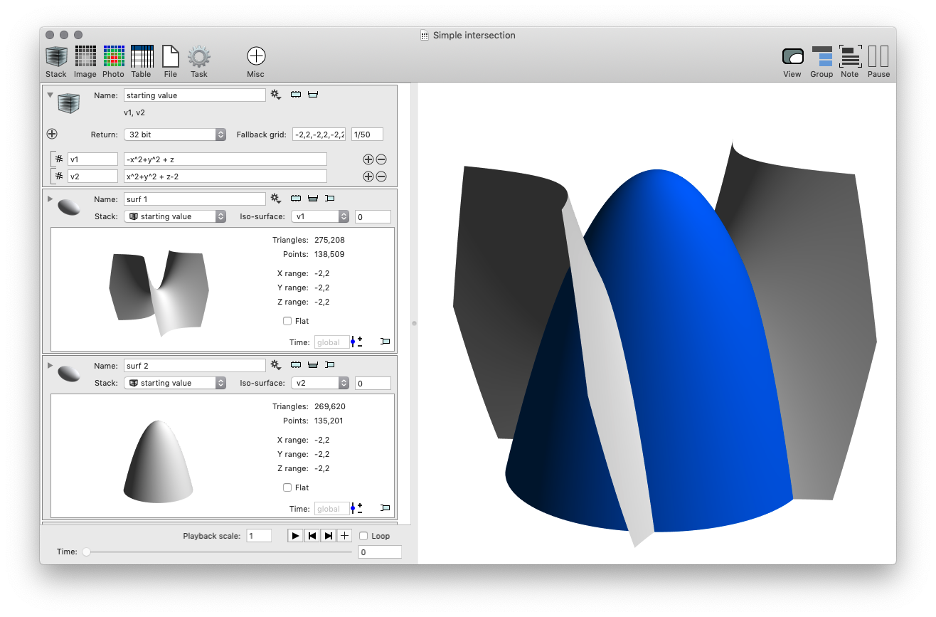
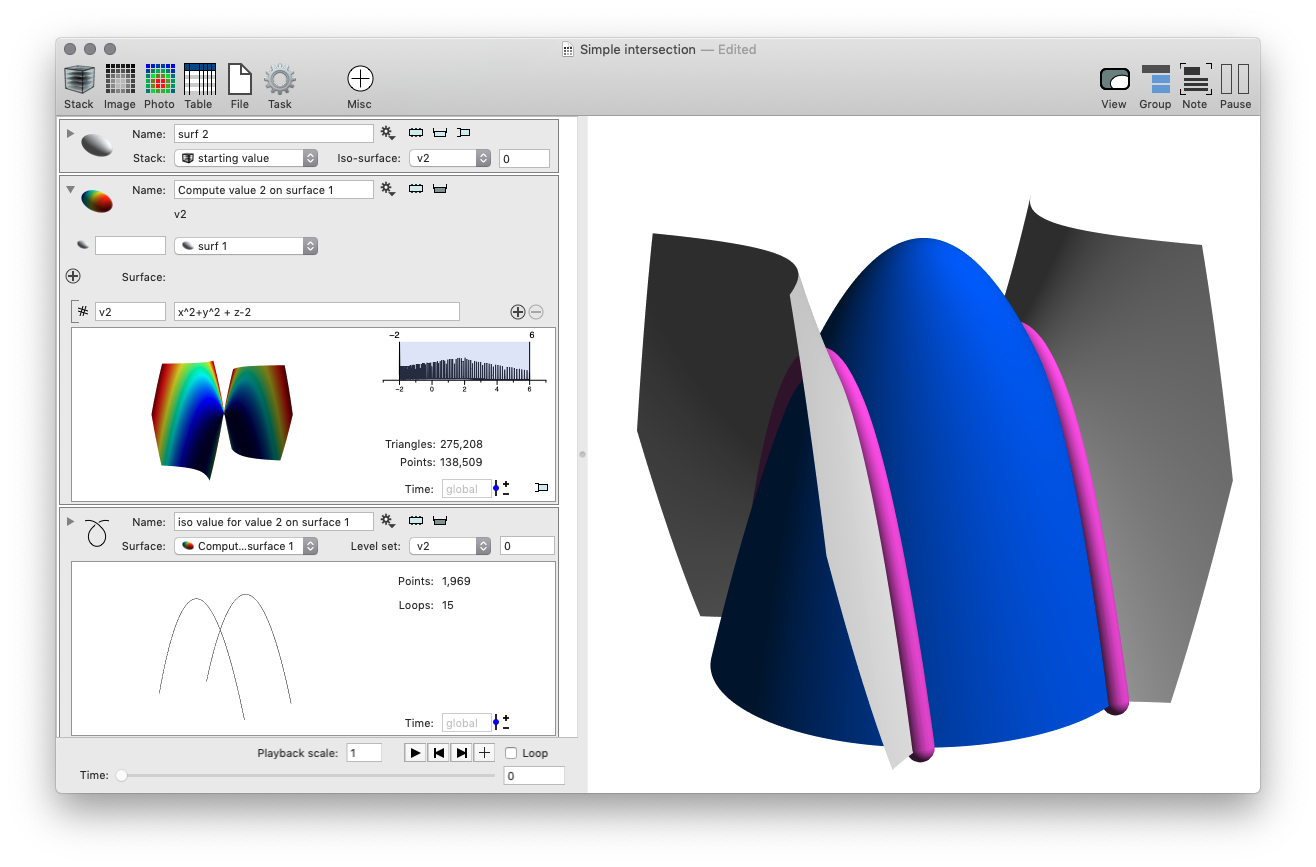
First compute the two fields on a uniform grid. This is done through the Image Stack Computation followed by a thresholded surface, two of them.
When you draw them together in a 3D graphic you will get something like this.
Curve Intersection
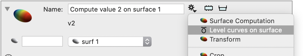
To find the intersection between these two surface, we use a slight trick, The surface computation allows you to evaluate an expression on a surface. This is similar to the image variable in that you can have one or more channels defined. In fact it creates a Surface Values Computation just like the Image Stack Computation that was used at the beginning. The surface is already added as a local variable. This gives you a x,y,z coordinate for each vertex and the expression is evaluated at each point. We take the first surface and evaluate the field from the second surface at those points in space. This is more accurate than interpolating the image stack on the surface, but that can be done also using the gear menu for the image stack.
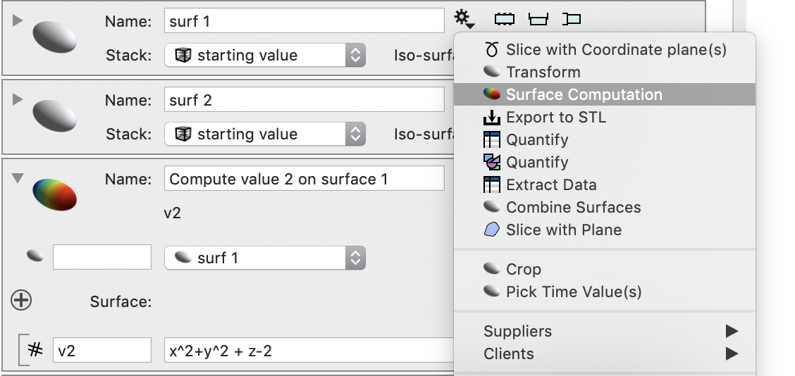
Now the intersection is where this value is zero. The value for the first expression is zero along all of the points on the surface because the surface is a zero level set of the first expression. That is done by using the gear menu again.
Now draw this path as well
Volume intersections
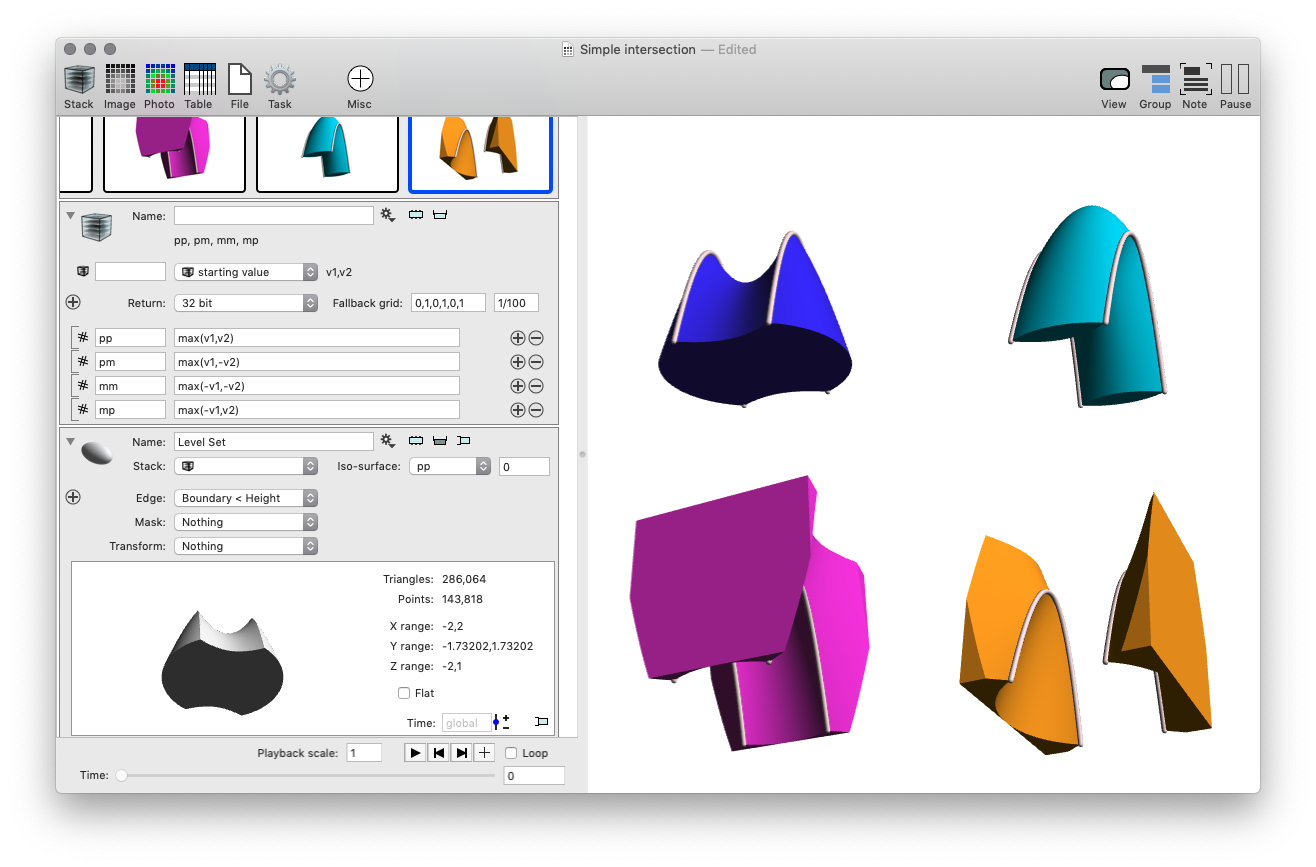
We can use the image stack computation to compute max of +/- of the two different scalar fields for an interesting effect. Take the thresholded surface for each channel.
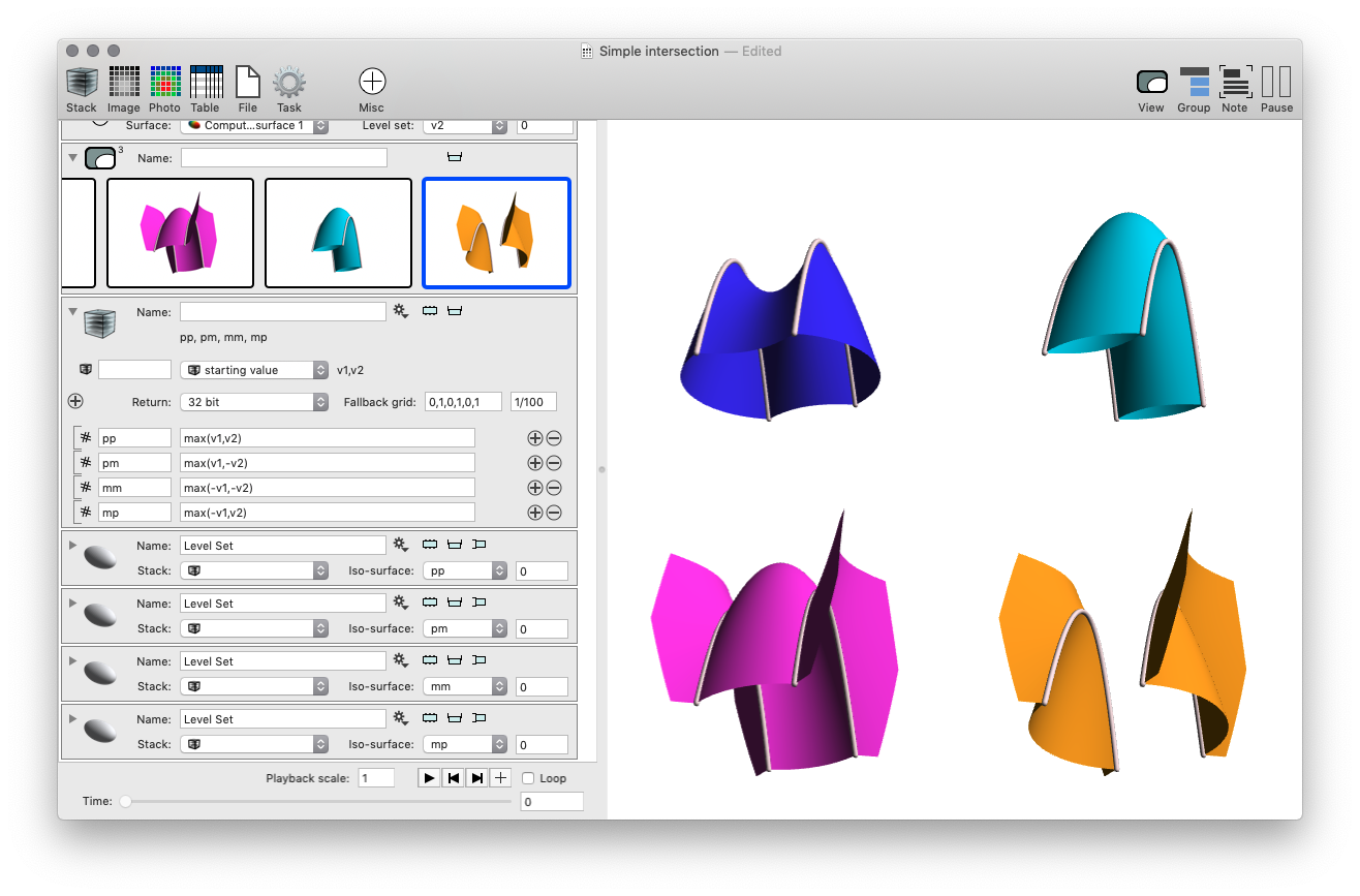
To close the solid, you need to go into one of the iso-surface finders and select the edge to include the boundary where the value is < height, i.e. negative.