Convergence test

Summary

Many numerical methods depend on a parameter like step size or grid size and the smaller the step size the higher the accuracy. Running a convergence test and determining the order of the method is a good way to verify that you implemented a numerical method properly and see if it works for your particular problem.

At a high level we have the following problem. Solution S(h) can be computed for a number of decreasing h values. Then E(S(h)) measures the error of this solution. The order is then determined such that E(S(h)) = Ch^p for some order p and constant C that will not depend on h.

What we need to do is to set up a sequence of tasks, run them all, gather the result and fit the data using a power function. The task is implemented using an external program.

Model problem

To make the code simple, we implement the Trapezoid method to approximate the integral of a function f on an interval [a,b] using N intervals. This gives you the step size h, h = (b-a)/N. Not every h is possible, since it needs to break the interval [a,b] into even sizes. The equation is

h(f(a)/2 + f(a+h) +f(a+2h) + … + f(b-h) + f(b)/2)

The error is then the difference between S(h) and the actual integral of f from a to b.

Time sequence

ImageTank has the concept of a time sequence. The slider at the bottom of the window is used to scrub through these values. By default there is no time dependence so this slider is disabled.

Every variable can have a time dependence, and when you use a time dependent variable as input, the output will be time dependent, except for a few actions, like the sampling method that we will use later.

Time values are non-negative and distinct, but don’t have to start at 0 or have a uniform stride. More information about this, and how time values are read from input sources like movies etc is explained elsewhere, but here we use the time sequence to create a sequence of inputs. The time values for this sequence will be 0,1,2,3,… but you can look at it as a zero based index for the collection.

Creating a Sequence

Create a new Group. Add a local variable (+ button) and select the “Add time sequence”

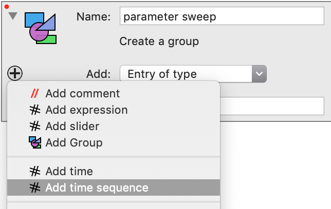
This adds a variable, wich by default is called t. This time is uniformly spaced in time and you specify the start, stride and what is the last time value. That means that if the stride is 1 and the last time value is 30 that you have 31 time values. If the stride is 0.5 you have 61 time values and the value for t is 0,0.5,1.0 etc.

This local variable can then be used in an expression inside the group. At this point you can vary the slider between 0 and the largest time value, which is 30. Note that if you specify time between values, like 9.34… the time value that will be used is at time 9. At that time 1.2^t = 1.2^9 = 5.15… which rounds to 4 and therefore N=9 as well. At t=30 this is up to 241.

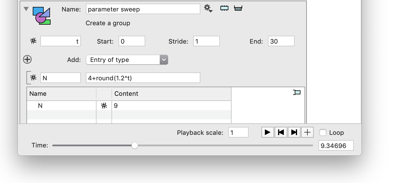
This means that the “parameter sweep” variable now has a time dependence, and when we use it for an argument for a program that will have time dependence as well.

Code for S(h)

We need to specify inputs. We could add these entries to the first group, but here we specify a different group that only has one time value and contains information about interval and function as well as the integral/anti-derivative of the test function. That will be used to compute the error later, but will not be handed over to the external program. Putting them in one group makes it easy to run different experiments.

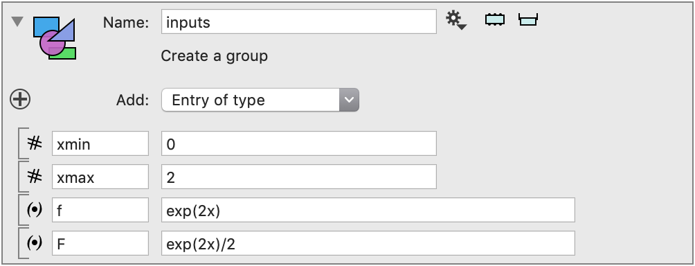
Now we are ready for the external task. This task should return the integral, and to make things simpler the external task also returns the step size. The external task needs the function and the interval from the second group, but the number of intervals, N, from the first group.

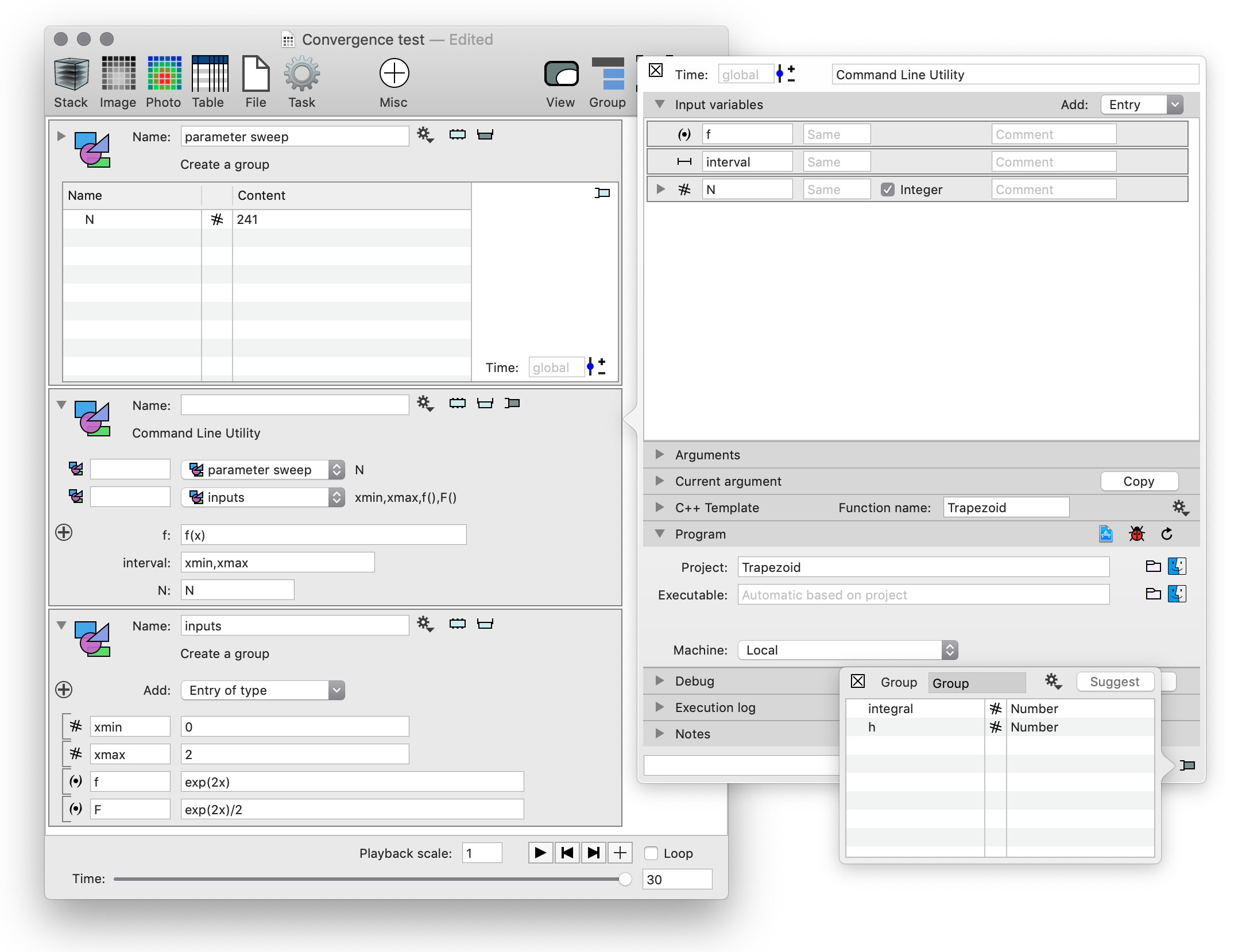
There are a number of things going on in this task definition.

• The output is two numbers, the actual integral and the step size that was used by the program.
• In the external program side bar you are handing in three variables, an analytic function, range and an integer. These are all entry fields and not variable selectors.
• In the input, the + button in the top left corner was used to add in two groups. Neither group has a name, but as the list to the right of the menu selection indicates, they add three numbers and two functions as local variables for this object.
• The local variables are used to specify the arguments.
• Since the “parameter sweep” object is time dependent the object becomes time dependent in the same way. That means that there are 31 different time values for the output.

The code is pretty simple, just copy paste it into the Xcode project. Note that the function name is specified.

Group Trapezoid(const DTFunction1D &f,DTRegion1D interval,int N)
 {
     double h = (interval.maxV-interval.minV)/N;
     double sum = (f(interval.minV)+f(interval.maxV))/2.0;
     
     for (int i=1;i<N;i++) {
         double x = interval.minV + i*h;
         sum += f(x);
     }
     sum *= h;
     
     Group toReturn;
     toReturn.integral = sum;
     toReturn.h = h;
     return toReturn;
 }

The error is then just the difference between the integral returned from this group and the actual integral, F(xmax)-F(xmin)

Sampling (h,E(S(h))

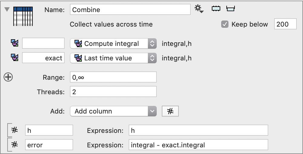
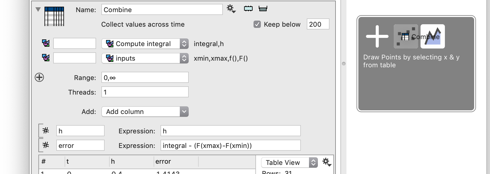
The next step is to compute the error and accumulate this across all of the runs. Since this is really a time series of entries the action here is to combine them into a table, where each record comes from a time value.

The object that is created already has the group connected so that it adds local variables. You also need the interval and an anti-derivative of f, and that is in a different group, so add this as input.

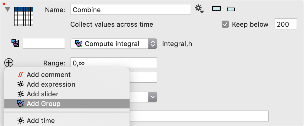
Specify two numerical columns and create expressions for each one. The first one is just h, the other one is the error.

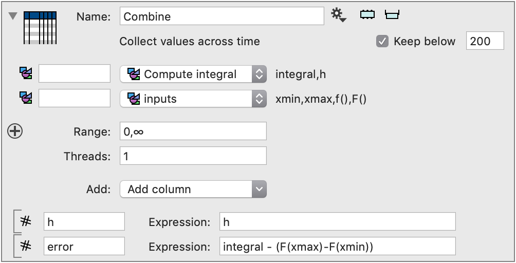
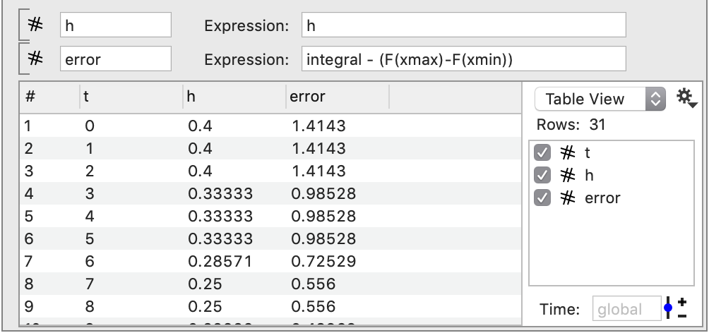
At each time value this defines a record, and this is combined in time to create a table. The time value is always included. When this table is used, ImageTank will handle the sampling for you and combine the results. Clearly the N value didn’t increase quickly in the beginning so the same step size was computed a few times.

Fitting the result

Start by drawing the result in a figure. Click and drag the icon of the table onto the right side of the ImageTank window. You need to widen the window for this to show up. When you get to the blank side you see a floating window pop up. Drag the icon onto the command you want to create. Here we want to draw the result as points.

You see a graph, but this is the second column as a function of the first column, i.e. h(t) and that is not what we want to draw. Go to the top left corner of the graph and click on the side bar icon

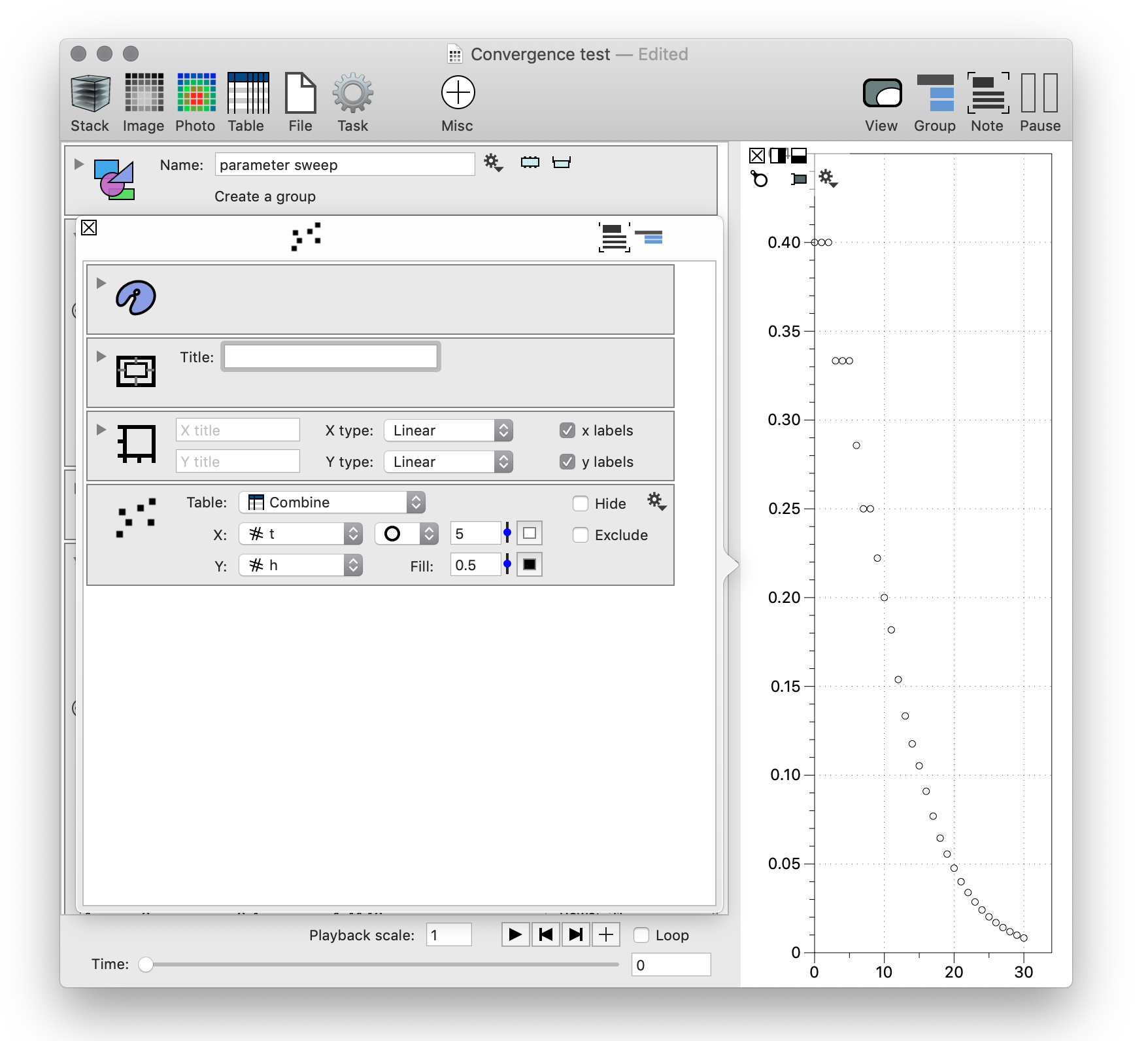
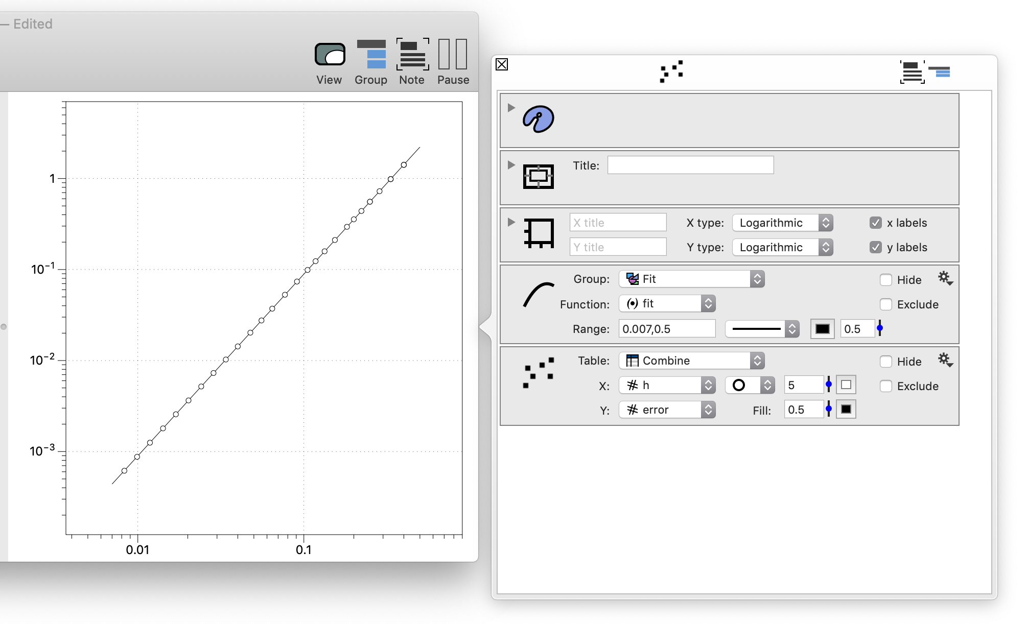
In the Points command, change x to h and y to error, and in the axis settings just above the Points command switch both the x and the y axis to logarithmic.

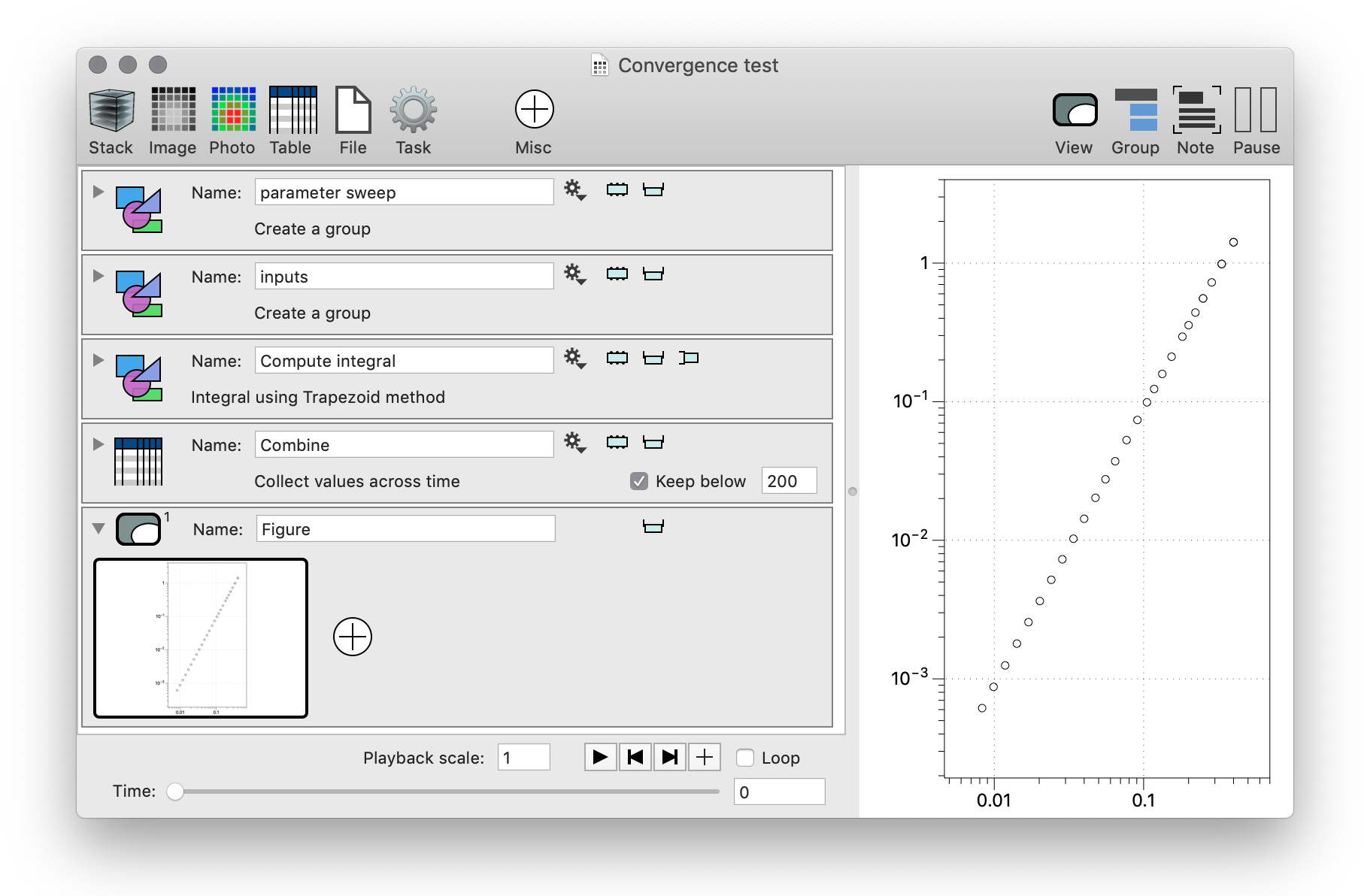
This is consistent with the rule error = Ch^2, for when h goes from 0.01 to 0.1 the error goes from about 10^(-3) to 10^(-1)

This is not quantitative enough however, so we need to compute a power fit and overlay that. To compute the power fit, select the Analyze columns action from the gear menu.

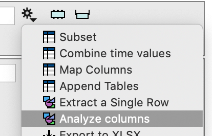
And then add a standard fit function

This entry allows you to select from the most common fits, linear, low order polynomial, exponential and power fit.

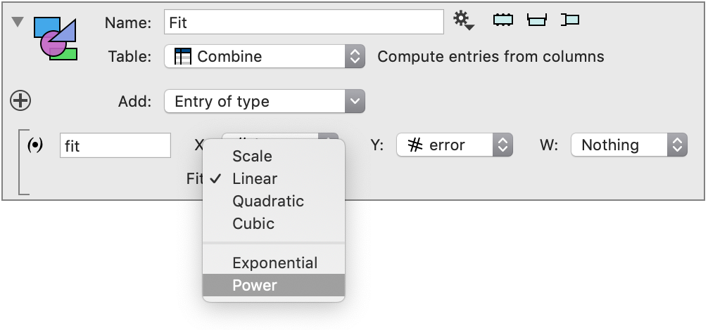
You can open up the variable monitor to see the result

And drag this over to the existing graph to add it to the graph. Note that you need to drag the Function command so that it is above the Points command. Otherwise the function goes over the points.

Unknown integral

If you don’t know the integral, i.e. the anti-derivative function F you can’t use the above method to compute the error. One way to do this is to estimate the exact solution and subtract that. You can do that with a different and more accurate method such as Simpsons or Gaussian Quadrature. You can also use the finest approximation to estimate the error.

The time sequence mechanism is used to set up a collection of parameters. The last time value is the smallest step size. We can pick up that time value by using the gear menu.

The time doesn’t have to match exactly. Given a time T what is returned is the largest time value t such that t≤T. If T is ∞ this means that you get the last time value.

When you combine the errors you include this last time as well as the computed time. Since the entry names match you need to give the approximation for the exact solution a prefix, such as “exact”. Then the expression becomes integral-exact.integral.