ImageTank Intro – Images
ImageTank structures computation in terms of variables/objects and displays them in various ways. This article explains how to create and display an image. It also goes over the concepts and building blocks that are used in ImageTank.
Create an Image
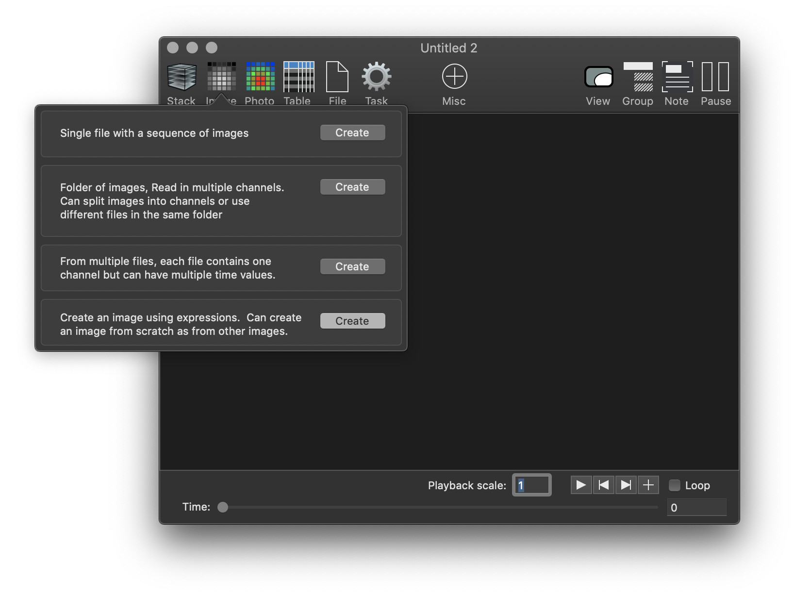
In the window toolbar you have a number of buttons to create objects. Each object has a variable type. In the pop-up window below you have four different ways to create an Image object. They each present different sets of options. These objects can then be used by other objects. ImageTank is strongly typed, and later we will use this image to compute a path variable. That object requires the input to an Image variable, but it doesn’t matter how that image is computed. Click on the last entry to create an image using expressions.
Using expressions
The image variable has one or more channels. The image is located in space and has an origin (x0,y0) and grid size dx and dy. This means that the pixels don’t have to be square. This is slightly different from what you are used to for bitmaps. Gray scale bitmaps can be viewed as an image with a single channel, and color images as images with three or more channels, red, green and blue, and possibly a transparency channel.
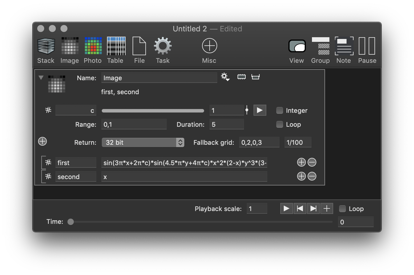
In this case we want to create two channels and call them “first” and “second”. To create an additional channel, click on the + icon in the lower right corner. The following expression is a little tricky
sin(3π*x+2π*c)*sin(4.5π*y+4π*c)*x^2*(2-x)*y^3*(3-y)
x and y are understood, and are the grid locations. c however is not yet defined which is why the expression for the first channel is red, there is a small red dot next to the icon for the first channel and there is a red dot in the top left corner. Those red dots are a UI queue that something is wrong and that the variable is currently not valid. Once fixed the error will go away.
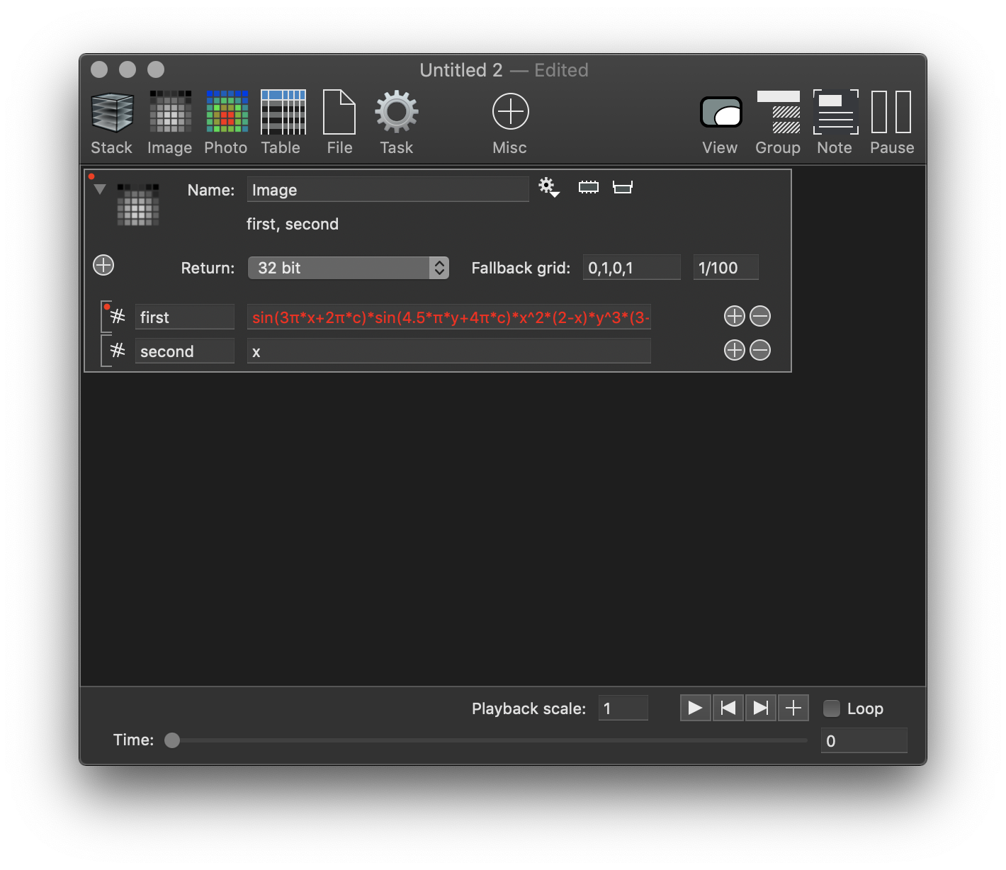
Before we fix this, note that just above where you specify the expression for the channels there is a menu that says “32 bit” and next to that a fallback grid. Images can be 8bit, 16 bit, float (32 bit) and double (64 bit). This is the resolution of each channel. Typically a bitmap will have a 8 bit resolution for each channel which is an integer between 0 and 255. 32bit and 64 are decimal numbers and are not rounded. The fallback grid is used because you are not using an image as input. The field 0,1,0,1 is for xmin, xmax, ymin, ymax. Change that to 0,2,0,3 so that you use the box [0,2]x[0,3]. The step size is 1/100 which results in a 201×301 array.
Adding a variable
“c” is the parameter we want to vary. Let’s break the following expression down.
sin(3π*x+2π*c)*sin(4.5π*y+4π*c)*x^2*(2-x)*y^3*(3-y)
The last part “x^2*(2-x)*y^3*(3-y)” has the property that it is 0 on the boundary of the box and positive on the inside. Because of the power “^2” and “^3” it isn’t symmetric and is flatter close to (0,0). The first part is the product of “sin(3π*x+2π*c)” and “sin(4.5π*y+4π*c)”. These are waves in “x” and “y” with different frequencies and then a phase shift “2π*c” and “4π*c“. We want “c” to be a parameter between 0 and 1 that we can vary. Click on the “+” button on the left hand side.
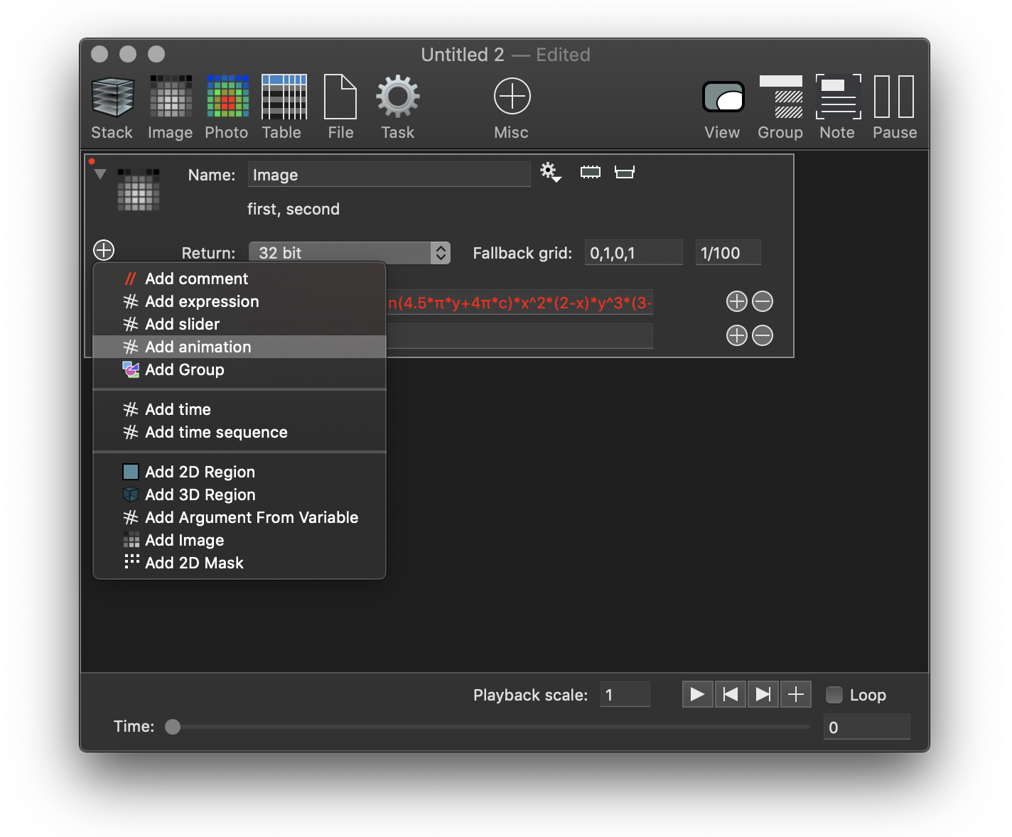
This menu adds local variables to the objects. These variables can then be referenced in expressions. At the bottom you can see that you can add a reference to an Image variable, but we won’t use that here. Instead select the animation option. Give this variable the name “c”. As soon as you do you can see that the expression for the first channel is understood and the red dots go away. The variable is now defined.
Viewing the image
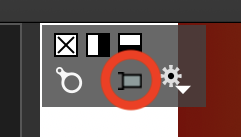
The simplest way to see the image you have is to click on the variable monitor button. This button is at the top of the object, to the right of the name. In the screen shown below you will see that it is a little darker once you press it. Every variable has a variable monitor and it shows an inspector for that variable type. The monitor is added to the bottom of the object, and you can toggle the variable monitor on and off. The disclosure triangle in the top left corner closes the detailed view and shows you just the first two lines of the object, but that is independent of the variable monitor.
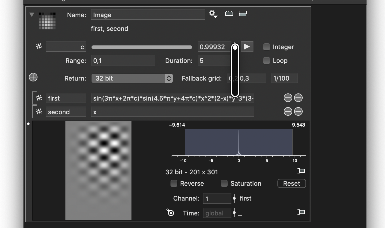
To change the animation variable you can type in a new value or click on the small slider image to the right of the numerical field. This uses the range you specified and can be interactively changed. Note changing the field updates the image live.
ImageTank is a multithreaded by design which allows the use of all processor cores. New Apple Silicon computers are 8 cores and will soon feature higher core counts. This is why you can still interact with the UI during execution. This is different from most programming environments where you set things up, hit run and then have to wait for that to finish before you can compute anything else. ImageTank computes automatically and concurrently. The small dot that flashes when processing indicates that this is being done in a separate thread, and as we will see later there will be a lot of these “busy dots” popping up when multiple cores are computing at the same time.
Drawing Views
The variable monitor is just an inspector. This is intended as a quick viewer, and not something for creating output images. You don’t have a lot of control over the representation. To do that widen the ImageTank window. It will add a vertical splitter. Now drag the image over to the right hand side. You do that by clicking on the icon in the top left corner, hold down the mouse and drag it. If you just click on the icon and release the mouse the object gets a blue border to indicate that it is selected.
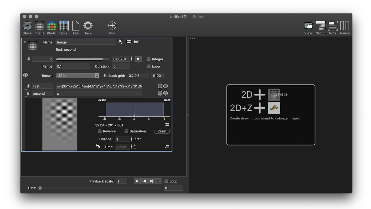
When you drag it over the right hand side you see two entries, one labeled 2D and the other 2D+Z. Lets start with the 2D view. Drag the image over the small icon to the right of the plus button so that it highlights. For some variable types you have more than one graphical representation and in that case you will see more than one icon. The icons are for drawing commands that will draw the varible.
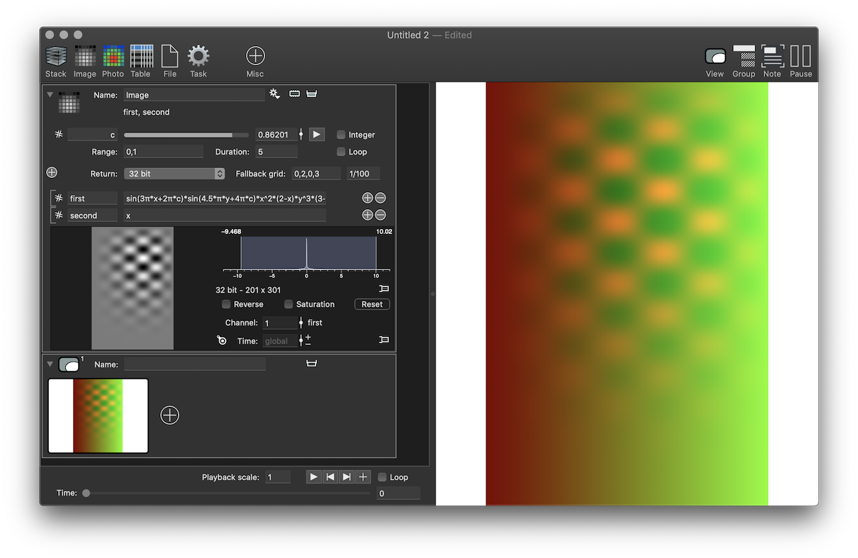
Two things happened. The right hand side now draws the image, but much more colorfully than the variable monitor. There is also a new entry below the image object. This new object is a View controller. Currently it just has a single view, but it can have multiple views, and you can have multiple view controllers.
Drawing Commands
Move your mouse to the top left corner of the graphic. This pops up a small floating window. On the second line in the middle, between the magnifying glass and the gear menu you see the side panel icon. Click on that.
That pops up a floating window attached to the right hand side if there is space for it there. Otherwise the left hand side. You can also hold down the option key to force it to be on the left hand side.
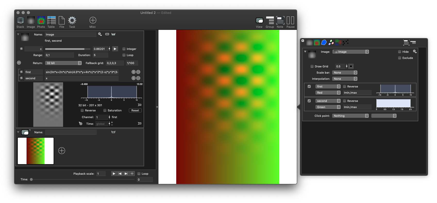
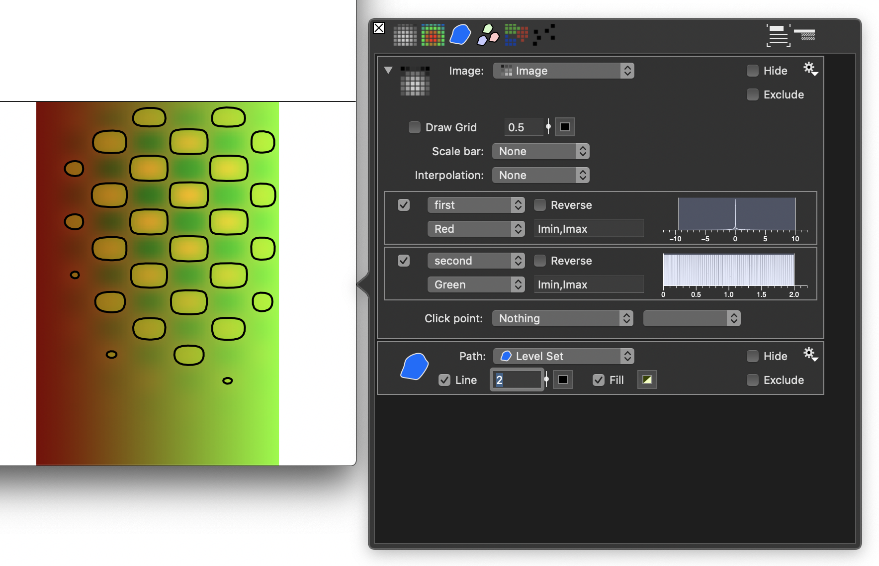
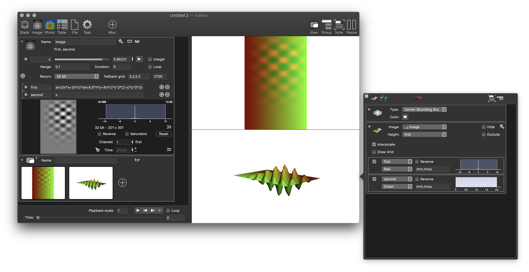
Currently this window only has one drawing command, to draw the image. It can have a number of drawing commands and they will be drawn as layers from bottom to top. You can click on hide or exclude to remove them from the drawing without deleting the drawing command. This command draws both channels, using the red and green channels. You can change the channel, coloring range, hide channels, etc. At the top you see which image variable is being displayed. If this file had more than one image you can choose between them. You can also draw multiple images and they will be drawn according to their location in space.
Draw in 3D
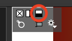
In one of the steps above you might have noticed the 2D+Z option. This draws the image in 3D using the value of one of the channels as the height. This uses Metal, Apple’s GPU renderering language, to draw the surface. To draw both at the same time, we start by splitting the view
Then drag the image to the 2D+Z option in the lower part.
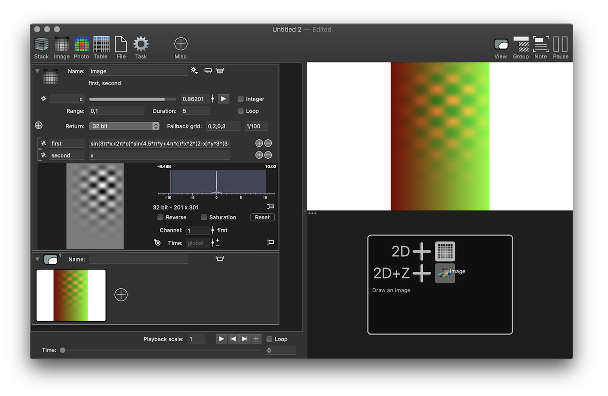
You can split the drawing area vertically and horizontally and resize by dragging the separators. The thumbnails in the view controller will stay even if you click on the close button in the popup. You need to click on the close button in the thumbnail to remove the graph. This allows you to set up a number of graphs and pick which one is displayed and where. The thumbnail also updates when the graph updates or you rotate the three dimensional image.
Adjusting the coloring
The coloring uses a blending model. For each channel you specify a color ramp and the final color is the maximum in each color channel. That means that if one is blue and the other green if both are fully saturated you get magenta. You can also pick the rainbow color ramp to get a spectrum of colors, even though this can be misleading and should be used carefully.
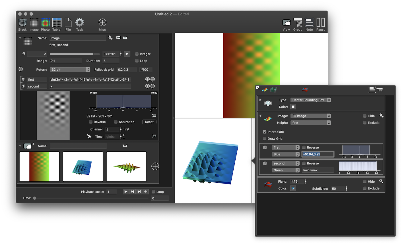
The above figure also has a semi-transparent plane. Add that by clicking on the small plane icon at the top of the pop-up window.
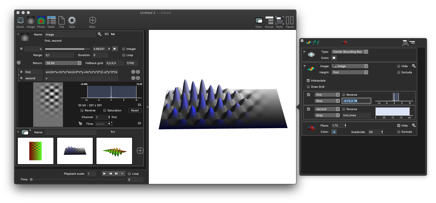
Here is an example where one channel is gray scale and the other is blue. The range for the blue coloring is adjusted so that only the tops are blue the rest are black and therefore do not affect the gray scale from the first.
Add a computation
All of the above examples just use one object, and show three ways to draw it, the variable monitor and two and three dimensional graphical representations. The real power of ImageTank comes from computing derived quantities from data, compositing raw and computed data in the same graph and exporting the result as figures and movies. That will take more time to explain, but to give a hint of that and show the main concepts take the example of computing a contour, often called a level set. Given a value, find the locations where the intensity is equal to that value, using interpolation to find a higher quality representation than a pixelated mask.
There is a large number of operations built into ImageTank, and you can add your own using external programs. Next to the name is a gear menu. This is a context sensive menu. The image variable has a number of actions and we pick the “Thresholded Path” from the list. As you can see from the icon in front of the entry this will create an object with a different variable type.
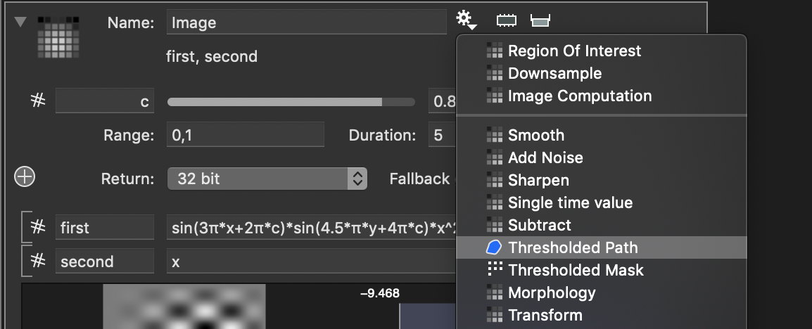
This creates the object and connects the image as input, just like was done in the drawing commands. You pick which channel you want to use for the threshold, and if you open the details you have more options and can add local variables. What you also see in this object, but not in the object that computes the channels is the side panel button. This brings up a mini applet with a user interface to help you set values quickly.
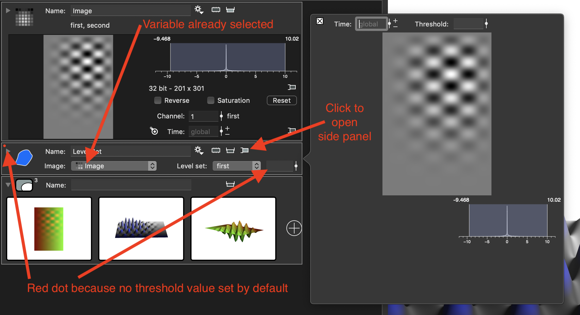
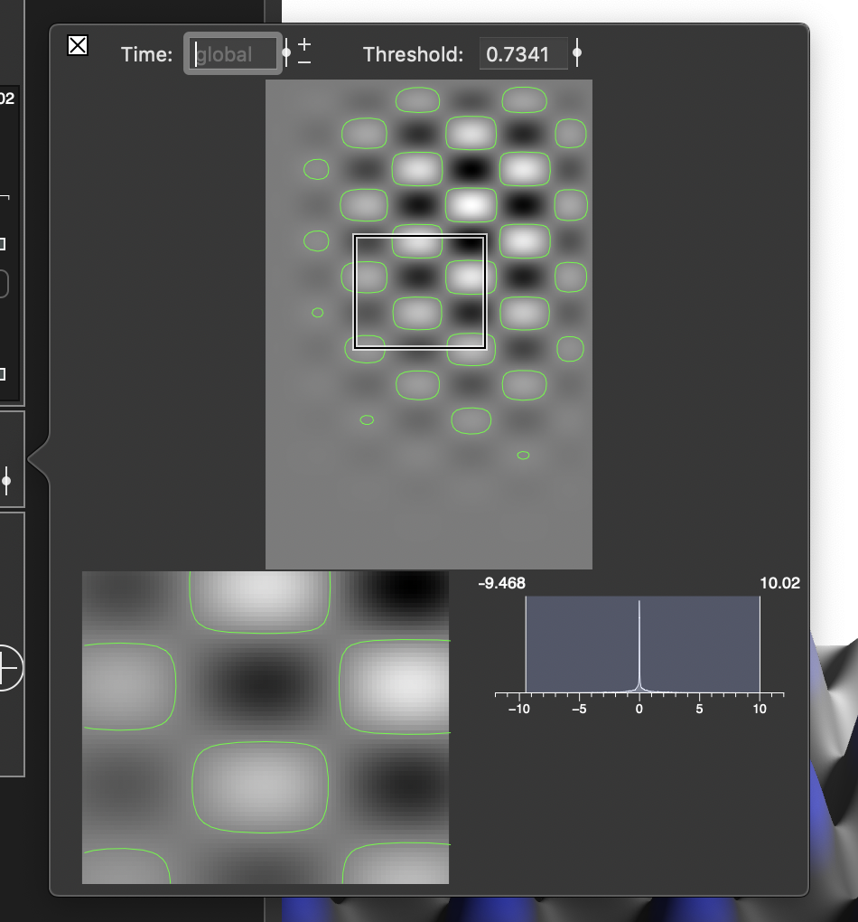
When you use the slider next to the threshold here, ImageTank will use the range of the current image and overlay the thresholded value on the channel. You can zoom in by clicking and dragging to focus on smaller details.
Close this side panel when you don’t need it anymore, you can always go back to it later. Drag the path onto the two dimensional graphic to overlay it.
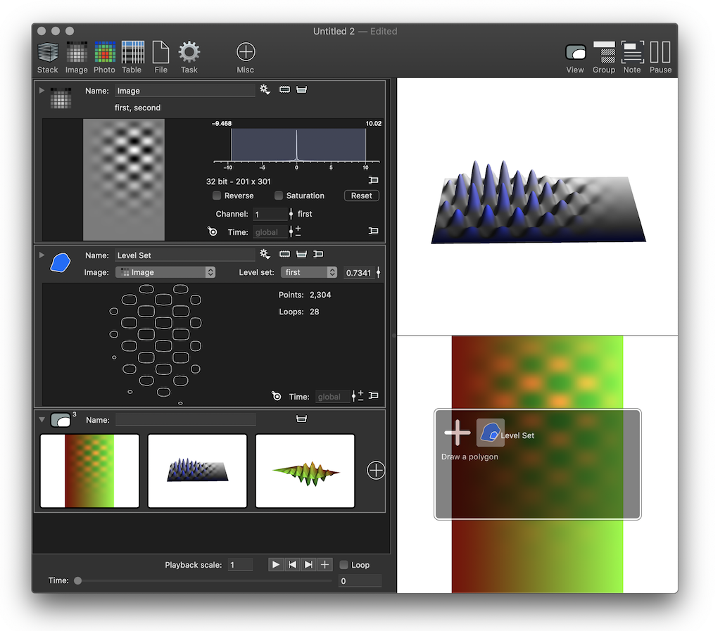
Here you have a lot more options for drawing the path layer.